Dexset

The Complete Guide to Training Data for Vision-Language-Action (VLA) Models (2026)

Five billion image-text pairs sit in LAION-5B (arxiv.org/abs/2210.08402); just over one million robot trajectories sit in Open X-Embodiment, the largest open robot dataset ever assembled (arxiv.org/abs/2310.08864). Those two numbers should not both describe the training diet of a single model family, yet every production VLA pairs a vision-language half fed at web scale with an action half starved at roughly one-thousandth of it. That mismatch, more than any architecture choice, is the defining constraint of physical AI in 2026.

The gap exists because the two halves come from different worlds. The vision-language half was pretrained on image-text pairs that already existed. The action half needs robot trajectories that do not exist until someone physically collects them, frame-synchronized, action-labeled, and paired with language instructions. You cannot scrape your way out of that. Which is why, on most VLA programs, the architecture question gets settled in a week and the compute budget in a month, while the question of how many language-annotated trajectories the model needs, at what task diversity, on which embodiments, goes unanswered the longest.

This guide gives you the full picture: what VLA training data is, how the landmark models (RT-1, RT-2, OpenVLA, Octo, pi-zero, GR00T) actually sourced their data, how action representation changes your labeling requirements, what collection and annotation cost per hour, and how to scope a dataset that transfers to your embodiment instead of overfitting to someone else’s lab. The thesis we argue throughout, and the one our delivery data keeps confirming: once you stand on the open-data base layer, dataset composition (task diversity, instruction diversity, capture fidelity) predicts VLA capability better than episode count, so budget should follow distribution, not volume.

DexSet supplies egocentric, exocentric, teleoperation, mono, and stereo data to robot foundation model teams. The numbers in this guide come from our own rigs, QA pipelines, and cost benchmarks, alongside the primary papers. Where a figure is our internal benchmark rather than a published result, we say so.

TL;DR: Key Takeaways – VLA training data consists of robot trajectories (synchronized camera frames + robot actions) paired with natural-language instructions, usually collected via teleoperation. – Landmark scale points: RT-1 used ~130k episodes over 17 months; OpenVLA pretrained on ~970k episodes from Open X-Embodiment; pi-zero reports on the order of 10,000 hours of dexterous robot data. – Action representation drives labeling spec: discrete action tokens (RT-2, OpenVLA) tolerate lower control rates; continuous-action heads (pi-zero flow matching, Octo diffusion) reward 50 Hz, low-jitter capture. – In our benchmarks, teleoperation collection runs $28-60 per robot-hour depending on rig and task complexity; a proper language annotation pass adds $8-15 per hour of data. – Data mixture beats raw volume: co-training on web-scale vision-language data plus a well-balanced robot mixture is what gives VLAs semantic generalization. – Task and scene diversity predict generalization better than episode count once you pass a per-task floor (roughly 50-150 demonstrations per task in the imitation-learning literature).

What Is Training Data for Vision-Language-Action (VLA) Models?

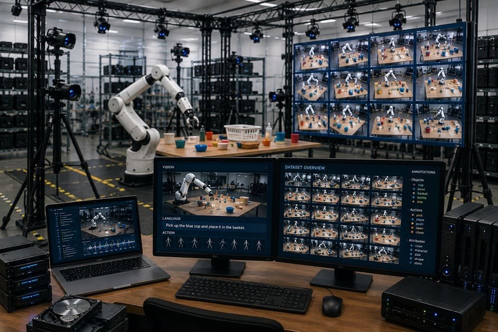
Training data for VLA models is a corpus of robot demonstration episodes in which each timestep pairs visual observations, robot proprioceptive state, and executed actions, and each episode (or segment) carries a natural-language instruction describing the task. A VLA model consumes images and an instruction as input and produces robot actions as output, so its training data must contain all three aligned in time.

A single well-formed episode contains:

  • Observations. One or more camera streams (wrist-mounted, over-the-shoulder exocentric, or head-mounted egocentric), typically 224×224 to 1080p RGB at 10-60 fps, optionally stereo pairs or depth.
  • Proprioception. Joint positions, gripper state, end-effector pose, usually at the control rate.
  • Actions. The command stream that produced the motion: delta end-effector poses, joint targets, or gripper commands, timestamped against frames.
  • Language. An instruction such as “put the red mug on the top shelf,” attached at episode level, and increasingly at sub-episode segment level for long-horizon tasks.

The entity chain matters for anyone mapping this space: teleoperation rigs (ALOHA-style leader-follower arms, VR controllers, exoskeletons) produce demonstrations; demonstrations feed imitation learning; imitation learning at scale, on top of a pretrained vision-language backbone, is what turns a VLM into a VLA. The Hugging Face LeRobot project has become the de facto open format for storing these episodes, and its dataset cards are a good reference for what a clean schema looks like.

How the Landmark VLA Models Sourced Their Data

Every major VLA result is downstream of a specific, documented data strategy, and the strategies differ more than the architectures do. Reading the data sections of these papers teaches you more about building a VLA than reading the model sections.

Model (Year)OrgParamsRobot DataLanguage SourceAction Representation
RT-1 (2022)Google35M~130k episodes, 13 robots, 17 months, ~700 tasksTemplated instructionsDiscrete tokens, 256 bins (arxiv.org/abs/2212.06817)
RT-2 (2023)Google DeepMind12B / 55BRT-1 data, co-fine-tuned with web-scale VLM dataTemplated + web textActions as text tokens (arxiv.org/abs/2307.15818)
Octo (2024)UC Berkeley et al.27M / 93M800k trajectories from Open X-EmbodimentMixed, dataset-dependentDiffusion head, continuous (arxiv.org/abs/2405.12213)
OpenVLA (2024)Stanford et al.7B970k episodes from Open X-EmbodimentMixed OXE instructionsDiscrete tokens (arxiv.org/abs/2406.09246)
pi-zero (2024)Physical Intelligence~3BOn the order of 10k hours, 7 platforms, 68 task familiesNatural + segment-level relabelingFlow matching, 50 Hz continuous (arxiv.org/abs/2410.24164)
GR00T N1 (2025)NVIDIA2BData pyramid: web video + synthetic + real robot dataMixed human + generatedContinuous, diffusion-based (arxiv.org/abs/2503.14734)

Three lessons sit in that table. First, scale climbed from 130k episodes to roughly a million in two years, but the biggest capability jumps (RT-2 over RT-1, pi-zero over Octo-class models) came from mixture changes, not just volume. Second, OpenVLA at 7B outperformed the 55B RT-2-X on the paper’s 29-task evaluation suite, which tells you curated cross-embodiment data can substitute for an order of magnitude of parameters. Third, nobody serious trains on robot data alone anymore; co-training against web-scale vision-language corpora is standard because it is what keeps semantic knowledge (what “the leftmost ripe banana” means) alive while the model learns motor control.

Core Data Modalities for VLA Training

Modality choice determines what your VLA can learn and what your collection rig must capture. The main axes are viewpoint (egocentric vs exocentric), depth strategy (mono vs stereo), and collection method (teleoperation vs human video).

Egocentric vs Exocentric Views

Egocentric data is captured from the robot’s or demonstrator’s own viewpoint; exocentric data is captured from external cameras watching the workspace. Wrist and head cameras give the policy view-invariant, occlusion-realistic inputs and tend to transfer better across scene layouts. Exocentric views give annotators and QA reviewers the context to verify task success and label segments. In our pipelines we treat exocentric streams as partly a QA instrument: an episode with only a wrist view is roughly twice as expensive to verify because reviewers must scrub proprioception logs to confirm success.

Mono vs Stereo

Mono capture records a single RGB stream per viewpoint; stereo capture records calibrated pairs that support depth estimation. Most published VLAs train on mono RGB because the backbone VLMs are mono. Stereo earns its extra cost on contact-rich and clutter-heavy manipulation, where depth ambiguity is a dominant failure mode. Our rule of thumb: mono for pretraining breadth, stereo for the fine-tuning set on your target tasks.

Teleoperation vs Human Video

Teleoperation produces the gold standard because the action stream is the robot’s own. Leader-follower rigs like ALOHA (arxiv.org/abs/2304.13705) hit high dexterity at a hardware cost around $20k per station; VR-based rigs are cheaper and faster to train operators on but add pose-retargeting noise. Human egocentric video (Ego4D, EgoExo4D scale) has no action labels, so it enters VLA training as a co-training or pretraining signal, the approach GR00T N1 formalizes as a data pyramid. Human video buys you visual and behavioral priors cheaply; it never replaces the teleop layer where actions live.

Action Representation: Tokenization vs Continuous Actions

Action representation is the choice of how robot actions are encoded for the model to predict, and it silently rewrites your data spec. There are two dominant families.

Discrete action tokenization (RT-1, RT-2, OpenVLA) bins each action dimension, typically into 256 buckets, and treats action prediction as next-token prediction. It plugs directly into a language-model backbone and tolerates modest control rates. The FAST tokenizer (arxiv.org/abs/2501.09747) pushed this further with a compression-based scheme that makes autoregressive VLAs viable on high-frequency data.

Continuous action heads (Octo’s diffusion head, pi-zero’s flow matching) regress action chunks directly. They excel at dexterous, high-rate control (pi-zero runs 50 Hz) but they punish sloppy capture. Timestamp jitter between frames and actions that a tokenized model shrugs off will smear a flow-matching target distribution.

What this means for data buyers, from our QA logs:

  • For tokenized targets, 10-15 Hz aligned capture is usually sufficient; invest the savings in task diversity.
  • For continuous heads, capture at 30-60 Hz with hardware-timestamped sync; we hold frame-to-action skew under 10 ms on our teleop rigs because beyond that we can measure it in fine-tune loss.
  • Action-chunk prediction (introduced with ACT on ALOHA) means episodes must be free of teleoperator pauses mid-chunk, which is a QA check most teams add only after their first bad fine-tune.

Language Annotation: The Layer Everyone Underestimates

Language annotation is the process of attaching instructions to robot episodes, and it is where VLA datasets most often quietly fail. A VLA is only as language-conditioned as its labels are diverse.

Templated vs natural instructions. RT-1-era datasets used templates (“pick X”, “move X near Y”). Templates are cheap and consistent, and they teach the model a grammar of about a dozen verbs. Models trained on templated instructions follow paraphrases poorly; the semantic generalization RT-2 demonstrated came from the web co-training, not the robot labels. Current practice, visible in the pi-zero and DROID (arxiv.org/abs/2403.12945) pipelines, is natural free-form instructions plus paraphrase augmentation.

Episode-level vs segment-level labeling. Episode-level labeling attaches one instruction to a whole demonstration. Segment-level labeling breaks a long-horizon episode into sub-tasks (“open the drawer”, “place the spoon inside”, “close the drawer”) with aligned timestamps. Segment labels cost more but unlock long-horizon training and better credit assignment. In our pipeline, segment-level labeling costs roughly 2.5x the episode-level pass because annotators must scrub video and mark boundaries, not just watch and describe.

Our first-hand benchmark: a language annotation pass adds $8-15 per hour of robot data depending on instruction density and whether we run single or dual annotation. We also run an instruction diversity QA gate: across any 1,000-episode batch we require minimum thresholds for unique verbs, unique object references, and spatial-relation phrases, because we have watched fine-tunes on label-poor batches lose the ability to follow anything but the majority phrasing.

Data Mixtures, Co-Training, and Cross-Embodiment Transfer

A data mixture is the weighted combination of datasets a VLA trains on, and mixture design is now a first-class engineering discipline. Three decisions dominate.

Web co-training ratio. RT-2 established that co-fine-tuning on web vision-language data alongside robot data preserves semantic breadth. Teams that fine-tune on robot data alone consistently report the model “forgetting” open-vocabulary grounding.

Cross-embodiment weighting. Open X-Embodiment showed that pooling data across 22 robot types improves average success, and OpenVLA and Octo both hand-tuned per-dataset mixture weights rather than sampling uniformly. Transfer across embodiments is real but not free: it appears strongest between similar morphologies (single-arm manipulators with parallel grippers) and weakest into dexterous hands and humanoids, which is exactly why humanoid programs still commission embodiment-matched collection.

There is no published universal mixture ratio, and be suspicious of anyone who quotes one. What the papers do agree on is the shape of the curve: heavily downweight any single dataset that would dominate by timestep count, keep a meaningful web co-training fraction throughout fine-tuning rather than dropping it to zero, and upweight the small datasets that match your target embodiment and camera geometry. In practice we see teams land between 10% and 40% embodiment-matched data by timestep in their final fine-tuning mixtures, with the exact point set by held-out evaluation rather than by principle. Measure mixtures in timesteps or tokens, not episodes; episode lengths vary enough between sources that episode-level accounting quietly misstates composition by 2-3x.

Diversity vs depth. Once a task passes a demonstration floor (Mobile ALOHA showed strong results co-training with as few as 50 demonstrations per task on top of a broad base, arxiv.org/abs/2401.02117), the marginal episode of task 12 is worth less than the first episode of task 13. When we rebalance client collections, we usually shift budget from episode count toward scene, object, and instruction diversity, and the downstream evaluations reward it.

Cost and Economics: What VLA Training Data Actually Costs

VLA data cost is driven by four stacked line items: rig amortization, operator time, annotation, and QA. Vendors who quote a single opaque per-episode price are hiding this stack. Here is ours, from DexSet production benchmarks (round figures, typical ranges we see):

Cost ComponentTypical RangeNotes
Teleop collection (VR rig, tabletop tasks)$28-38 per robot-hourIncludes operator, station amortization, resets
Teleop collection (leader-follower, bimanual/contact-rich)$40-60 per robot-hourALOHA-class rigs, slower resets, higher operator skill
Language annotation, episode-level$8-10 per data-hourNatural instructions, single pass
Language annotation, segment-level + paraphrases$12-15 per data-hourTimestamped sub-task boundaries, dual pass on 10%
QA and success verification$5-9 per data-hourSuccess labels, sync checks, instruction diversity gate
Useful episodes per collection hour20-40 tabletop; 8-15 long-horizonAfter discarding failed/aborted episodes

Worked example: a 2,000-hour bimanual manipulation corpus with segment-level language and full QA lands between $114k and $168k. Against that, note that pi-zero-class results were built on roughly 10,000 hours. This is why mixture design and cross-embodiment pretraining matter commercially: nobody fine-tuning a foundation model should be paying to recollect the base layer that OXE-scale open data already provides. Pay for the embodiment-matched, task-matched, well-labeled top of the pyramid.

Case Study Proof: Scaling a Fine-Tuning Corpus for a Humanoid Team

A humanoid foundation model team came to us with an OpenVLA-style base model and a fine-tuning problem: strong tabletop scores, weak performance on their bimanual kitchen tasks, and instructions that only worked when phrased like the training templates. We scoped a 1,400-hour teleoperation collection across 42 task families with a hard instruction-diversity requirement (no template allowed to exceed 8% of a batch) and segment-level labels on all long-horizon episodes.

The mixture, not the volume, did the work. Their prior corpus had 3x our episode count but 9 task families and 14 instruction templates. After fine-tuning on the new corpus blended 60/40 with their legacy data, their internal evaluation showed task success on held-out kitchen tasks roughly doubling, and paraphrased-instruction success moved from near-random to parity with template phrasing. We report those as directional results from the client’s own evaluation harness, not audited benchmarks. The full breakdown is in our case study write-up.

Scoping Your Own Collection: The RFP Scorecard

A VLA data RFP scorecard is a structured checklist for comparing data vendors on the dimensions that predict fine-tune quality. If you take one action from this guide, make vendors answer these in writing:

  • Frame-to-action sync tolerance, in milliseconds, with measurement method.
  • Control and capture rates, and whether timestamps are hardware or software.
  • Instruction sourcing: templated, natural, or paraphrase-augmented, with a diversity metric per batch.
  • Episode-level vs segment-level labeling, priced separately.
  • Success-labeling protocol and inter-annotator agreement.
  • Cost per robot-hour, broken into collection, annotation, and QA. Refuse bundled per-episode pricing.
  • Delivery format (LeRobot-compatible schemas save your team weeks).

We publish ours as a downloadable template. [Download the VLA Data RFP Scorecard] and use it against us too.

Related reading this week:

Next Step

If you are scoping a VLA data collection this quarter, two options. Book a demo and we will walk through our teleop rigs, annotation pipeline, and the instruction diversity QA gate live. Or download sample data: a free LeRobot-format sample pack of bimanual teleop episodes with segment-level language labels, so your team can inspect sync quality before you talk to anyone.

Frequently Asked Questions

What is training data for vision-language-action (VLA) models?

It is a corpus of robot demonstration episodes pairing synchronized camera observations and robot actions with natural-language instructions. VLA models train on it, usually via imitation learning on top of a pretrained vision-language backbone, to map images plus an instruction to robot actions.

Pretraining-scale efforts use hundreds of thousands of episodes (OpenVLA used ~970k from Open X-Embodiment; pi-zero reports on the order of 10,000 hours). Fine-tuning an existing VLA to a new embodiment or task set typically needs far less: the literature shows meaningful results from 50-150 demonstrations per task on top of a broad base, with 500-2,000 hours being a common commercial fine-tuning corpus.

In DexSet’s benchmarks, teleoperation collection runs $28-60 per robot-hour depending on rig and task complexity, language annotation adds $8-15 per data-hour, and QA adds $5-9. A 2,000-hour fully annotated corpus typically lands between $110k and $170k.

Not for most pretraining, since mainstream VLA backbones consume mono RGB. Stereo or depth earns its cost on contact-rich, cluttered, or precision tasks in your fine-tuning set, where mono depth ambiguity is a leading failure mode.

Only partially. Human egocentric video has no robot action labels, so it serves as a pretraining or co-training signal (the GR00T N1 data pyramid approach), improving visual and behavioral priors. The action-labeled teleoperation layer remains mandatory for the policy to output executable control.

Tokenized VLAs (RT-2, OpenVLA) discretize each action dimension into bins and predict actions as tokens, which suits language-model backbones and moderate control rates. Continuous-action VLAs (pi-zero with flow matching, Octo with diffusion) regress action chunks directly, enabling 50 Hz dexterous control but demanding tighter timestamp sync in the training data.
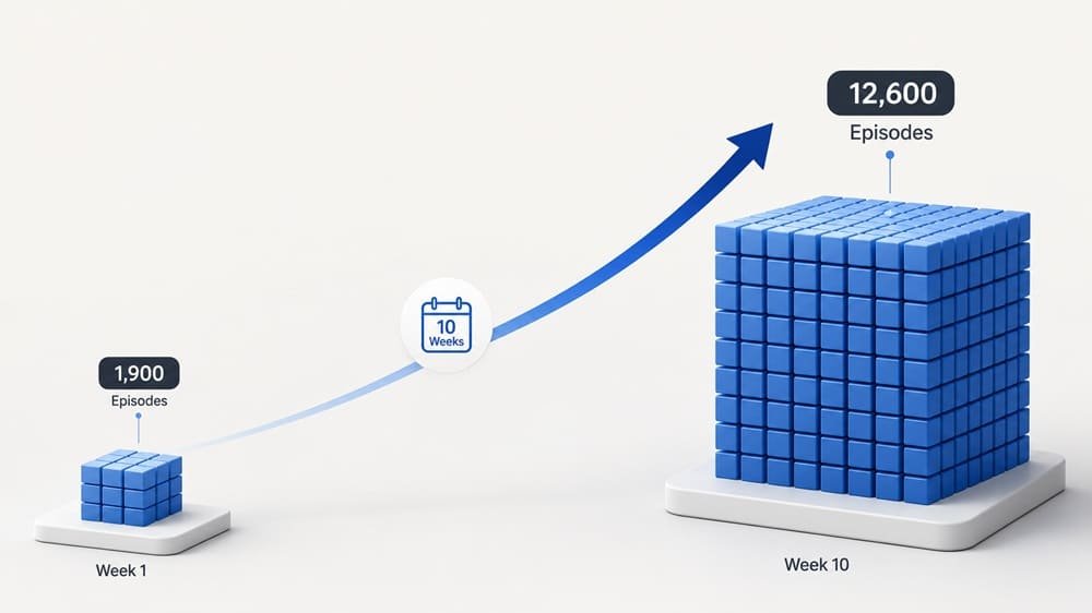
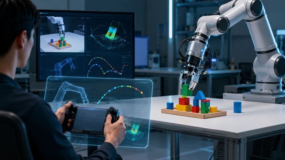
Case Study: Scaling Teleoperation Data for a VLA Model, 1,900 to 12,600 Episodes in Ten Weeks

A head of data once asked us which of their 1,900 collected episodes had actually made their policy better, and we could not tell them; neither could they, because nothing in their pipeline had ever connected episodes to outcomes. That question came from the team this case study is about: eight weeks into their own collection effort, 1,900 episodes against a 12,000-episode target, a 34 percent QA rejection rate, and a training deadline that had already slipped once. Their ML team was strong. Their collection operation was two engineers moonlighting as floor managers, and it showed.

This is the common failure shape, and it is the thesis of this case study. Collection stalls not because anyone lacks skill but because demonstration data is an operations problem wearing an ML costume: staffing, ergonomics, and QA gating, none of which appear in the papers. The papers do tell you what is possible; ACT hit 80 to 90 percent success from about 50 clean demos per task (arxiv.org/abs/2304.13705). Getting 12,000 clean demos across 40 tasks is a different discipline.

Here is exactly what we changed, week by week, including the two things that failed. Use it as a template for your own program, or as an argument for not running one in-house.

Key Takeaways – Baseline: 1,900 episodes in 8 weeks, 34 percent rejection. Outcome: 12,600 QA-passed episodes in 10 weeks, 12 percent final rejection. – Six leader-follower stations plus a two-week operator certification program did most of the work. – Automated ingest QA (sync skew, smoothness, completion gates) cut silent data loss to near zero. – Client’s ACT baseline improved from 41 to 68 percent average success across their internal 40-task eval. – Peak steady-state: about 1,400 usable episodes per week from 8 operators.

The Starting Point: Why 1,900 Episodes Took Eight Weeks

The client’s bottleneck was a stack of small losses, not one big one. Their audit told the story: two VR stations shared among rotating volunteers, no defined operator roles, no reset protocol, and QA performed manually by an ML engineer, at training time, weeks after collection. Rejection ran 34 percent, dominated by timestamp skew between their 50 Hz action logs and 30 fps cameras, plus inconsistent initial states that made half the “passing” episodes weak training signal anyway.

Their effective yield was under 60 usable episodes per day. At that rate the 12,000-episode target sat more than eight months out.

What We Changed

The intervention had four parts: stations, people, protocol, and gates. In order of impact:

1. Stations. We replaced the two shared VR rigs with six bimanual leader-follower stations (GELLO-class leaders on the client’s arms, roughly $300 per leader plus fabrication), keeping one VR station for the mobile-base tasks where it fit better. Joint-level control cut trajectory hesitancy immediately and shortened operator ramp.

2. People. Eight dedicated operators on a two-week certification program: task cards, reset drills, and a throughput gate (20 usable episodes per hour on a reference task) before touching production tasks. Our standard ramp curve applied; novices started at 8 to 12 usable episodes per hour and certified operators stabilized at 25 to 40.

3. Protocol. Written task cards for all 40 tasks, marked randomization zones for object placement, success criteria defined at collection time, and per-episode metadata (task, operator, rig, success) attached at the source.

4. Gates. Automated ingest QA running nightly: inter-stream sync skew over 33 ms flagged, dropped-frame counts, jerk thresholds on joint trajectories, and completion labels verified against a sampled human review. Failures routed back to the floor as next-morning feedback per operator, which mattered as much as the gate itself.

The Week-by-Week Numbers

Weekly usable output tells the ramp story better than any narrative.

Week Usable episodes Rejection rate Notes
1 310 29% Station bring-up; operators in certification
2 540 26% First cohort certified; jig redesign after reset failures
3 980 19% All 8 operators on production tasks
4 1,390 15% Steady state reached
5 to 9 1,300 to 1,450/wk 11 to 14% Two task cards rewritten after eval feedback
10 1,280 12% Target passed: 12,600 total QA-passed

Two failures worth admitting. In week two, our first reset jig for a deformable-object task increased reset time instead of cutting it; operators beat the jig by hand and we scrapped it. And one of the 40 tasks, bimanual jar opening, ran a stubborn 25 percent rejection until week six, when slowing the commanded demonstration pace fixed what better hardware had not.

Did the Data Actually Help? Policy Results

The point of episode counts is policy performance, so the client re-trained their ACT baseline on the new corpus at week eleven. Average success across their internal 40-task evaluation went from 41 percent (trained on their original 1,900 mixed-quality episodes) to 68 percent, with the largest gains on precision tasks where the old VR data had been noisiest. Same architecture, same hyperparameter budget, different data. Their team’s summary, which we will keep quoting: “We spent six months on model changes for less improvement than ten weeks of better data.”

That is one program, not a controlled study, and we flag it as such. But it matches the pattern across our floors and the published record: demonstration quality moves policy success more reliably than architecture iteration at this stage of the field.

What We Would Do Differently

Every program teaches something, and this one taught us three corrections we have since made standard. First, we would start the operator certification cohort a full week before station bring-up finishes, not after. Waiting for hardware serialized two ramps that could have run in parallel, and it cost the program most of week one’s output. Second, we would pilot every task card ourselves before handing it to operators. Two of the 40 cards contained ambiguous success criteria (“lid secured” without a torque or rotation definition), and the resulting label inconsistency did not surface until the week-five training run flagged suspicious loss on exactly those tasks. A ten-minute pilot per card would have caught both. Third, we would set the deformable-object tasks to a slower commanded pace from day one. The week-six discovery that pace, not hardware, drove the jar-opening rejection rate had been sitting in the per-task rejection data since week two; we were looking at floor-level averages and missed it. Per-task dashboards are now default on every program we run.

None of these are exotic lessons. That is rather the point: scaling demonstration data is a discipline of small, boring corrections applied early, and the gap between 1,900 episodes and 12,600 episodes was made of exactly such corrections.

The Reusable Checklist

Scaling teleoperation collection comes down to seven decisions made early:

  • Match rig to task family (leader-follower for fine bimanual work; VR for mobile/humanoid tasks)
  • Dedicated, certified operators, never rotating volunteers
  • A throughput gate before production collection
  • Written task cards with randomization zones and success criteria
  • Hardware timestamps on every stream; sync checked at ingest, not at training
  • Nightly automated QA with per-operator feedback loops
  • A rejection buffer of at least 15 percent in the episode target

Rig options, cost-per-episode math, and QA thresholds are covered in depth in the complete teleoperation data collection guide.

Next Step

Ready to scope your data program? Talk to our team.

Frequently Asked Questions

How many episodes does a VLA model program need?

Program-dependent, but the humanoid teams we support typically target 10,000 to 50,000 QA-passed episodes per quarter across dozens of tasks. Single-task ACT policies can work from about 50 clean demos; multi-task generalization is what drives volume.

With rigs, certified operators, and ingest QA in place, expect three to four weeks to steady state. This program reached about 1,400 usable episodes per week from 8 operators by week four.

At least 15 percent at maturity and 25 to 30 percent during the first two weeks of any new task or rig. Budgeting zero rejection is the most common planning error we see.

In-house costs more than teams expect once engineer time is counted; the client here spent eight engineer-weeks producing data that mostly failed QA. Outsourcing wins on time-to-data in most cases; in-house wins when collection is itself a core competency you intend to build.

Rig fidelity and QA gating together. Joint-level leader-follower control removed trajectory hesitancy, and ingest gates stopped skewed episodes from reaching training. Success rose from 41 to 68 percent with no model changes.

Teleoperation Data Collection for Robot Learning: The Complete 2026 Guide

Midway through a humanoid data program last year, our cost per usable episode rose almost 40 percent in a single week, and for two days nobody could explain it. Every rig passed its health checks. The QA gates were green. The answer had nothing to do with hardware or pipelines: two trained operators had left, their replacements were producing at novice rates, and the ramp math did the rest. Papers make demonstration collection look like a solved problem. In production, it is a staffing, hardware, and QA operation that most ML teams have never run before.

That week is this guide in miniature, and it carries the thesis the whole page argues: teleoperation data collection is an industrial operation, not an ML task, and it succeeds or fails on operational levers. It is part hardware engineering (leader arms, cameras, time sync), part human operations (hiring, training, and retaining operators), and part data engineering (formats, QA, versioning). Underestimate any one leg and the dataset comes out late, expensive, or unusable.

This guide covers the full stack: what teleoperation data collection actually is, the five main rig approaches and what they cost, the economics of operator labor, how demonstrations turn into trained policies, and the QA thresholds that separate usable datasets from expensive noise. The numbers on operator throughput, cost per hour, and rejection rates come from our own collection floors; the hardware and algorithm claims come from the primary literature (ALOHA, GELLO, UMI, DROID, Open-TeleVision), cited throughout.

TL;DR – Teleoperation data collection is the process of recording synchronized robot actions and sensor observations while a human remotely controls the robot through a task, producing demonstrations for imitation learning. – Five rig families dominate: leader-follower arms (ALOHA, ~$20k bimanual), low-cost kinematic leaders (GELLO, roughly $300 per arm), VR controllers/headsets (Quest 3, Vision Pro), 6-DoF desktop devices (SpaceMouse), and robot-free handheld capture (UMI). – Realistic all-in operator cost runs $28 to $60 per teleop hour. Novice operators produce 8 to 12 usable episodes per hour; trained operators reach 25 to 40 within two to three weeks. – Expect 10 to 30 percent QA rejection. Budget for it up front or your episode targets will slip. – 50 clean demonstrations trained with ACT reached 80 to 90 percent success on fine bimanual tasks in the original ALOHA work. Quality compounds; volume alone does not.

What Is Teleoperation Data Collection?

Teleoperation data collection is the process of recording a robot’s proprioceptive states, actions, and camera observations while a human operator remotely controls the robot through a task, producing time-aligned demonstration episodes used to train imitation learning policies. Each episode is a synchronized log: joint positions and velocities, commanded actions, gripper state, and multiple camera streams, typically stored in HDF5 or the LeRobot dataset format (github.com/huggingface/lerobot).

The entity chain matters for anyone mapping this space. Teleoperation produces demonstrations. Demonstrations feed imitation learning algorithms such as ACT (Action Chunking with Transformers, arxiv.org/abs/2304.13705) and Diffusion Policy (arxiv.org/abs/2303.04137). Those policies, scaled across tasks and embodiments, become the training substrate for vision-language-action (VLA) models. Open X-Embodiment aggregated over one million trajectories across 22 robot embodiments largely from teleoperated sources (arxiv.org/abs/2310.08864). No teleop data, no VLA.

A useful mental model: a teleop episode is worth exactly as much as its worst-synchronized stream. A 50 Hz action log paired with a camera that drifted 80 ms out of alignment teaches the policy that objects move before the hand does. That single failure mode wastes more training budget than any other we see.

Core Concepts and Data Modalities

A teleoperation dataset is defined by four things: the action space, the observation streams, the control and capture rates, and the episode structure. Get these right before collecting a single demo, because retrofitting a format after 10,000 episodes is miserable.

Action Space and Leader-Follower Mapping

Leader-follower joint mapping is the control scheme in which a human moves a small “leader” arm and a “follower” robot arm mirrors those joint positions in real time. ALOHA uses this directly: two WidowX-class leader arms drive two ViperX 300 followers, joint to joint, which gives operators immediate kinesthetic intuition and avoids inverse kinematics singularities (arxiv.org/abs/2304.13705). GELLO takes the same idea and rebuilds the leader from hobby-grade Dynamixel servos and printed parts for roughly $300 per arm (arxiv.org/abs/2309.13037). VR and SpaceMouse rigs instead command end-effector poses and rely on an IK solver, which is cheaper but introduces its own artifacts near joint limits.

Observation Streams: Mono, Stereo, Wrist, and Overhead

Observation streams are the camera and sensor feeds recorded alongside actions, and their placement determines what the policy can actually learn. The standard manipulation setup is one or two exocentric (scene) cameras plus one wrist camera per arm. Stereo pairs or depth add geometric grounding for tasks with occlusion. Our default rig records three RGB streams at 640×480, 30 fps, plus joint states at the control rate. Egocentric head cameras matter for humanoid teleop, where systems like Open-TeleVision stream an actively controlled head view into the operator’s headset (arxiv.org/abs/2407.01512).

Control Rate vs Camera Rate: The 50 Hz / 30 fps Problem

The rate mismatch problem is the timing gap created when actions are logged at 50 Hz but cameras capture at 30 fps, leaving no camera frame for two out of every five action steps. ACT-style pipelines handle this by training on the nearest or interpolated frame and predicting action chunks (sequences of 50 to 100 future actions) rather than single steps, which smooths over per-step jitter. What the algorithm cannot fix is unsynchronized clocks. Hardware-timestamp every stream at the source, log in one process or use a shared monotonic clock, and record the offsets. In our QA pipeline, any episode with inter-stream skew above 33 ms (one camera frame) is auto-flagged, and it is the single most common rejection reason on new rigs.

Episode Structure and Task Definition

An episode is one complete attempt at a defined task, from a randomized initial state to a labeled terminal state. Discipline here is what makes a dataset trainable: written task cards, explicit reset procedures, randomized object poses within a marked region, and a per-episode success label assigned at collection time. Datasets that skip initial-state randomization produce policies that memorize a table layout instead of learning a skill.

The Five Rig Approaches Compared

Rig choice is the decision that fixes your cost floor, your data quality ceiling, and which tasks you can collect at all. There is no universal winner; there is a right answer per task family and budget.

Approach Example system Hardware cost Control fidelity Operator ramp Best for Weakness
Bimanual leader-follower ALOHA (Stanford) ~$20k; Mobile ALOHA ~$32k with base Joint-level, 50 Hz, kinesthetic Fast (days) Fine bimanual manipulation Cost per station; fixed embodiment
Low-cost kinematic leader GELLO ~$300 per leader arm + robot Joint-level, high Fast Scaling stations cheaply on arms you own Build/maintenance effort; per-robot tuning
VR headset + controllers Quest 3 rigs; Open-TeleVision style $500 to $3,500 + robot Pose-level via IK, medium-high Medium (1 to 2 weeks) Humanoids, mobile manipulation, immersive tasks IK artifacts, some operator fatigue/sim sickness
6-DoF desktop device 3Dconnexion SpaceMouse $150 to $450 + robot Pose-level, low-medium Slow for contact-rich work Simple pick-place, lab prototyping Slow, unintuitive for dexterous or bimanual tasks
Robot-free handheld UMI gripper Under $1,500 per device Demonstrations without a robot Fast In-the-wild diversity, pre-robot data Embodiment gap; SLAM-dependent pose quality

Three field notes that the spec sheets miss. First, DROID, one of the largest open manipulation datasets (76,000 episodes, 350 hours, 564 scenes), was collected with a Meta Quest 2 controller driving a Franka arm, proof that consumer VR hardware scales to serious datasets (arxiv.org/abs/2403.12945). Second, GELLO is the highest-throughput-per-dollar option if you already own the follower arms, but plan for a part-time technician; printed leaders drift and servos strip. Third, UMI (arxiv.org/abs/2402.10329) is the only approach that collects before your robot ships, which makes it a strong hedge for teams still finalizing hardware.

For a deeper head-to-head, see our companion piece on comparing teleoperation approaches.

Economics: What Teleoperation Data Actually Costs

The true cost of teleoperation data is operator hours multiplied by an all-in rate, divided by usable episode yield, and most budgets get all three numbers wrong. Hardware is the smaller line item; a $20k ALOHA station running two shifts amortizes to under $3 per collection hour over a year. Labor and QA dominate.

Our first-hand benchmarks, consistent across programs we run:

Cost and throughput factor Typical range (our benchmarks)
All-in operator cost (wages, supervision, facility, hardware amortization) $28 to $60 per teleop hour
Novice operator throughput (weeks 1 to 2) 8 to 12 usable episodes per hour
Trained operator throughput (week 3 onward) 25 to 40 usable episodes per hour
QA rejection rate (mature pipeline) 10 to 15 percent
QA rejection rate (new task or new rig, first 2 weeks) 20 to 30 percent
Effective cost per usable episode roughly $0.90 to $6.00 depending on task complexity

Two implications fall out of that table. The operator ramp curve is a 3x throughput difference, so operator retention is a data-cost lever bigger than any hardware decision; churn resets you to novice yield. And QA rejection compounds against you: a 10,000-episode target with 25 percent rejection means collecting 13,300, not 10,000. We cover the bottleneck math in detail in why teleoperation data is the bottleneck in physical AI.

ROI framing for buyers: at $40 per hour all-in and 30 usable episodes per hour, a 50,000-episode dataset costs about $67k in collection labor before QA overhead. Compare that against three to six months of two ML engineers building and debugging an in-house collection operation, and outsourced collection frequently wins on time even when it ties on cost.

From Demonstrations to Policy: The Imitation Learning Pipeline

The imitation learning pipeline is the sequence that converts teleoperated demonstrations into an evaluated robot policy: collect episodes, convert to a training format, train ACT or a diffusion policy, then measure real-world success rate. The pipeline is short; the feedback loop is what teams underuse.

  • Collect and QA. Episodes stream into storage with per-episode metadata (task, operator, rig, success label). QA gates on sync skew, dropped frames, trajectory smoothness, and task success.
  • Convert. HDF5 or ROS 2 bags convert to LeRobot format for training and sharing on Hugging Face.
  • Train. ACT with action chunking (predicting ~100-step action sequences at 50 Hz) or Diffusion Policy for multimodal action distributions.
  • Evaluate. Fixed evaluation protocol: N rollouts per task with randomized initial states, report success rate.
  • Loop. Failure modes from evaluation define next week’s collection priorities.

The proof point worth anchoring on: the original ACT work reached 80 to 90 percent success on fine bimanual tasks such as cable routing and battery insertion from only 50 demonstrations per task (arxiv.org/abs/2304.13705). Demonstration quality and consistency, not raw volume, set that outcome. We have watched 400 sloppy episodes lose to 120 clean ones on the same task, same architecture. Collect less, reject more, retrain sooner.

Case Study Proof: Scaling a VLA Data Program

A humanoid foundation model team came to us needing 12,000 QA-passed bimanual episodes across 40 household tasks in ten weeks, after their in-house effort had produced 1,900 episodes in eight weeks with a 34 percent rejection rate. We stood up six leader-follower stations, ran a two-week operator certification program, and enforced automated sync and smoothness gates at ingest. By week four the floor was producing 1,400 usable episodes per week; the program closed at 12,600 QA-passed episodes with a 12 percent final rejection rate, and the team’s ACT baseline improved from 41 to 68 percent average task success on their internal eval. The full breakdown, including what failed in weeks one and two, is in the VLA case study.

Standing Up a Collection Program: The First 30 Days

A collection program launch is a 30-day sequence of hardware bring-up, protocol authoring, operator certification, and QA gate activation, in that order. Teams that compress or reorder it pay the cost back with interest in weeks five through eight. Our standard sequence:

Days 1 to 7: rigs and clocks. Assemble stations, calibrate cameras (record intrinsics and extrinsics per rig, per calibration), and prove time sync before anyone collects a demonstration. Log a physical sync event (a clapboard works) and verify every stream lands within one camera frame. A day spent here saves a re-collection later; skew discovered after 5,000 episodes is not fixable in post.

Days 8 to 14: protocol. Write task cards for the first five tasks: success criteria, reset procedure, randomization zones marked physically on the workspace, and expected episode duration. Pilot each card yourself before an operator touches it. Every ambiguity you leave in a task card becomes a labeling inconsistency in the dataset.

Days 15 to 28: certification. Run operators through reference tasks with a throughput bar (we use 20 usable episodes per hour) and a quality bar (QA pass rate above 80 percent) before production collection begins. Expect the standard ramp: 8 to 12 usable episodes per hour early, 25 to 40 after two to three weeks.

Day 30: gates on. Nightly automated QA becomes mandatory, with per-operator, per-rig reports every morning. From this point, the program self-corrects.

Build vs Buy: The Honest Decision Criteria

The build-versus-buy question comes down to whether demonstration collection is a competency your team needs to own or a supply problem it needs solved. Building makes sense in three cases: your embodiment is unusual enough that no vendor has matching rigs, your data requirements are small (under roughly 5,000 episodes), or collection know-how is itself part of your product thesis. Buying makes sense when the deadline is the constraint. The math from the economics section applies either way, but in-house programs carry two costs that rarely appear in the comparison spreadsheet: the two to four engineer-months of pipeline and QA tooling before the first reliable episode, and the management overhead of running an operations floor inside an ML organization. We are a vendor, so discount our view accordingly; then ask any team that has run both models which cost they underestimated.

Free Resource: Teleoperation Data RFP Scorecard

A vendor RFP scorecard is a weighted rubric for comparing teleoperation data providers on the criteria that actually predict dataset quality. Ours scores ten dimensions, including sync guarantees, QA rejection transparency, operator training programs, format deliverables, and per-episode pricing disclosure. Most vendors will not publish cost per hour; make them fill in the sheet. [Download the RFP scorecard (XLSX)] and use it on us too.

Related reading: 5 hidden challenges in teleoperation data collection.

Next Step

If you are scoping a demonstration data program, two options. Download 10 free teleoperation episodes (HDF5 plus synchronized MP4, three camera views, 50 Hz actions) and run them through your training stack. Or book a 30-minute scoping call with our data operations team and leave with a per-episode cost estimate for your task list. [Download Sample Data] | [Book a Demo]

Frequently Asked Questions

What is teleoperation data collection?

Teleoperation data collection is the recording of synchronized robot actions, joint states, and camera observations while a human operator remotely controls the robot through a task. The resulting episodes train imitation learning policies such as ACT and diffusion policies, which underpin VLA models.

Our all-in benchmark is $28 to $60 per operator hour, covering wages, supervision, facility, and hardware amortization. With trained operators producing 25 to 40 usable episodes per hour, effective cost lands between roughly $0.90 and $6.00 per usable episode depending on task complexity.

Fewer than most teams assume, if quality is high. The original ALOHA/ACT results reached 80 to 90 percent success on fine bimanual tasks with about 50 demonstrations per task. Multi-task and VLA training raises the requirement into the thousands per skill family, which is where collection economics start to dominate.

It depends on the task family and budget, per the comparison table above. Fine bimanual manipulation favors leader-follower rigs (ALOHA at ~$20k, or GELLO leaders at ~$300 per arm on robots you own). Humanoid and mobile tasks favor VR teleop. Robot-free UMI capture wins when hardware has not shipped yet.

The main causes are inter-stream time skew above one camera frame, dropped frames, jerky or hesitant trajectories, failed task completions, and reset protocol violations. Expect 20 to 30 percent rejection in the first two weeks on a new task and 10 to 15 percent once the pipeline matures.

Yes. UMI-style handheld grippers record demonstrations with a wrist-mounted camera and SLAM-derived poses, no robot required. The trade-off is an embodiment gap when transferring to your platform, so most teams use it to supplement, not replace, on-robot teleop.

HDF5 per episode and the LeRobot dataset format are the current de facto standards; ROS 2 bags are common at capture time. Whatever the container, require hardware timestamps on every stream and per-episode metadata (task, operator ID, rig ID, success label).

Why Exocentric & Multi-View Data Is the Biggest Bottleneck in Physical AI

Language models got their training data for free: by the time the first large transformer trained, the internet had already spent decades producing trillions of tokens describing every topic from millions of viewpoints. Physical AI inherits no such gift. Robot data must be manufactured episode by episode, and most of it has been manufactured the cheap way: one camera, no calibration record, no synchronization guarantees. Compute got cheaper, architectures converged, and the gap between what models could absorb and what capture pipelines produce kept widening.

The pattern shows up concretely in teams we work with. One VLA group spent six weeks tuning architectures against a plateau. Bigger backbone, longer action chunks, better augmentation. The success rate on cluttered scenes moved two points. Then they looked at their data and found the real ceiling: every one of their 90,000 episodes was recorded from a single camera, and 40 percent of failures happened in the exact frames where that camera could not see the target object.

This post makes the case that calibrated exocentric and multi-view capture, not model design, is the binding constraint on manipulation performance right now, and shows what closing the gap costs. The evidence comes from public datasets (DROID, Open X-Embodiment, Ego-Exo4D), the RoboMimic observation-space study, and our own capture benchmarks at DexSet, where multi-view teleoperation rigs are what we run every day.

Key Takeaways – Single-view episodes cap policy performance on occlusion-heavy tasks regardless of architecture; the failure is in the data, not the model. – DROID made two external stereo views plus wrist a hard protocol requirement across 76,000 episodes; Open X-Embodiment’s viewpoint chaos shows what happens without such a standard. – The bottleneck is operational, not scientific: calibration drift, sync skew, and 3-4x storage are why teams default to one camera. – Our benchmarks: DROID-style rigs cost $4,500 to $7,000 to build and $26 to $38 per operated capture hour; that premium is small against a wasted training run.

Why Single-View Data Caps Policy Performance

A single-view dataset gives the policy exactly one projection of the world per timestep, so any state the camera cannot resolve is unlearnable. Occlusion is the obvious case: the gripper approaches, the object disappears behind it, and the policy is now acting on memory and hope. Less obvious is spatial grounding. Language-conditioned instructions like “put the mug behind the plate” require scene geometry a close-cropped wrist view never encodes.

The RoboMimic study (arXiv:2108.03298) quantified the general point years ago: on identical demonstrations, changing the observation space, including camera views, materially changed imitation learning outcomes. Observation design is a first-order variable. Yet teams routinely treat it as fixed plumbing while sweeping learning rates for a month.

We see the ceiling directly in our ablations at DexSet. On tabletop pick-place and insertion tasks, moving from wrist-only to wrist plus one calibrated external view produced the largest single jump in success rate we have measured from any data intervention. Adding a second external view helped again on occlusion-heavy tasks. No optimizer change came close.

What the Big Datasets Already Decided

The major post-2023 collection efforts treat multi-view as a requirement, and that consensus is evidence in itself. DROID (arXiv:2403.12945) recorded roughly 76,000 Franka episodes across 564 scenes with two external ZED stereo cameras and a wrist ZED Mini on every single episode, extrinsics calibrated. The protocol did not permit single-view shortcuts, because the authors understood that scene diversity is worthless if the model cannot see the scene.

Ego-Exo4D (arXiv:2311.18259) went further for human demonstration data: over 1,200 hours of skilled activity captured simultaneously from Aria glasses and multiple stationary exocentric cameras, synchronized and calibrated, precisely so models can learn correspondences between first-person and third-person views. Anyone planning to pretrain robot policies on human video needs that pairing.

Open X-Embodiment (arXiv:2310.08864) is the counterexample that proves the rule. It aggregates over a million trajectories from 22 embodiments, and its camera configurations are heterogeneous: wrist-only here, one exo view there, different poses everywhere, extrinsics often missing. Teams pretraining VLAs on it spend real engineering time coping with viewpoint inconsistency. The lesson is not that aggregation is bad; it is that viewpoint standards are cheap at capture time and expensive to retrofit.

The Real Bottleneck Is Operational, Not Scientific

The reason most data is still single-view is not ignorance; it is that multi-view capture is an operations problem disguised as a shopping list. Buying three cameras takes an afternoon. Keeping their extrinsics valid, their clocks aligned, and their output QA’d across hundreds of sessions is the part that defeats teams.

Three costs dominate:

  • Calibration maintenance. Extrinsics drift when mounts get bumped, booms sag, or thermal cycles shift fixtures. Without per-session verification, drift silently corrupts weeks of data. Our gate is a 0.5 px reprojection error check on a ChArUco sweep at every session start.
  • Synchronization. Software timestamps drift across devices; PTP (IEEE 1588) or hardware trigger lines fix it, but only if someone engineers and monitors the sync path. We reject sessions with more than 10 ms cross-camera skew on manipulation work.
  • Storage and throughput. A 4-camera 1080p30 rig produces 0.8 to 1.5 TB per capture day in our pipelines. Multiply your single-view storage budget by three or four, then add QA review time.

None of this is research. All of it is why the bottleneck persists.

What Closing the Gap Costs

The honest comparison is single-view capture cost versus multi-view capture cost versus the cost of the training runs and engineering time the single-view ceiling wastes. Our benchmark numbers:

Item Single-View (Wrist or 1 Exo) Multi-View (2 Exo + Wrist) Delta
Rig build $1,500 to $2,500 $4,500 to $7,000 +$3,000 to $4,500 one-time
Operated capture $18 to $25 / hr $26 to $38 / hr +$8 to $13 / hr
Storage per capture day ~0.3 TB ~1.0 TB ~3x
Occlusion-heavy task ceiling Hard cap, architecture-independent Removed The point

For a 500-hour dataset, the multi-view premium lands around $4,000 to $6,500 in capture plus the one-time rig delta. One senior engineer spending six weeks fighting a data-imposed plateau costs more, and one full retraining run on data you have to recollect anyway costs far more. The full cost model, camera comparisons, and rig geometry options are in our pillar guide: The Complete Guide to Exocentric & Multi-View Data for Robot Learning.

How to Scale Multi-View Capture Without Drowning

Scaling multi-view data means industrializing the boring parts. The checklist we run internally:

  • Standardize one rig geometry (we default to DROID-style: two external stereo, one wrist) so calibration procedures and QA gates are identical across stations.
  • Gate every session on a two-minute calibration verification clip; reject on reprojection error > 0.5 px or sync skew > 10 ms.
  • Automate extrinsics logging into the episode metadata, so every frame carries its camera poses forever.
  • Budget storage at 3-4x single-view and decide codec and retention policy before capture starts, not after the first full disk.
  • Ablate camera count on your own tasks before scaling past three views; in our experience the fourth camera rarely earns its cost.

Run the Failure Analysis Before the Next Sweep

If your policy metrics have plateaued and your dataset is single-view, run the failure analysis before the next architecture sweep: tag failures by whether the target was visible at decision time. If occlusion dominates, the fix is capture. Book a demo and we will walk you through calibrated multi-view sample episodes from our production rigs, with the calibration and sync metadata included.

Frequently Asked Questions

Why is multi-view data considered the bottleneck in physical AI?

Because model architectures and compute have outpaced data quality: policies trained on single-view episodes hit occlusion and spatial-grounding ceilings that no architecture change removes, and calibrated multi-view capture is operationally hard enough that most existing datasets never provided it.

In DexSet benchmarks, a DROID-style rig costs $4,500 to $7,000 versus $1,500 to $2,500 for single-view, and operated capture runs $26 to $38 per hour versus $18 to $25. Storage roughly triples.

Standardize one rig geometry across stations, gate every session on calibration and sync checks, embed extrinsics in episode metadata, budget storage at 3-4x single-view, and ablate camera count on your own tasks before adding a fourth view.

DROID enforced two external stereo views plus wrist across 76,000 episodes; Ego-Exo4D paired ego and exo video across 1,200+ hours for cross-view learning; RoboMimic showed observation space choices materially change imitation outcomes; Open X-Embodiment shows the integration cost when viewpoint standards are absent.

No. In our ablations the second view delivers the largest gain, a third helps on occlusion-heavy tasks, and a fourth is rarely distinguishable from noise while adding roughly 25 percent to storage and QA cost.

Case Study: How We Scaled Exocentric & Multi-View Data for a VLA Model

We once shipped a pilot batch with an 18 millisecond wrist-camera clock offset, and this case study exists partly because of it. The mistake was ours: the wrist stream was timestamped off the arm controller instead of the rig’s PTP clock domain, invisible in playback, and it was the customer’s smoke-test training run at hour 20 that surfaced it. We fixed it, changed our rig standard, and kept the lesson. Vendor case studies that report zero mistakes are describing a project that never touched hardware.

This one covers eight weeks of work with a humanoid foundation model team (anonymized by agreement) whose manipulation policy had stalled on cluttered-scene tasks. The claim we will argue with the numbers below: their ceiling was informational, not architectural, and a disciplined multi-view capture operation, pilot batches, per-session calibration gates, one shared clock domain, is what removed it.

The team arrived with a specific complaint. Their policy trained fine, evaluated fine on open scenes, then dropped hard on cluttered tabletops. Their dataset: tens of thousands of teleoperated episodes, every one recorded from a single fixed camera. Failure review showed what you would expect. When clutter occluded the target from that one viewpoint during approach, the policy guessed.

They asked us for multi-view capture at a rate their internal rig could not hit: hundreds of hours within a quarter, calibrated, synchronized, and QA’d to a standard their ML leads could defend. What follows is how we built it, what it cost, what broke, and what the retrain showed. For the general framework behind these choices, the pillar guide is here: The Complete Guide to Exocentric & Multi-View Data for Robot Learning.

Key Takeaways – 600 hours of DROID-style multi-view episodes (two external stereo + wrist) delivered across 8 weeks on 4 parallel stations. – Per-session calibration gates rejected 4.1 percent of sessions; every rejection would have shipped corrupted extrinsics without the gate. – All-in capture cost landed at $31 per hour, inside our standard $26 to $38 benchmark range. – Retrained on matched episode counts, the customer’s occlusion-heavy split improved by double digits; open-scene performance held.

The Starting Point: Diagnosing a Data Ceiling

A data ceiling is a performance plateau caused by information missing from the training set rather than by model capacity. Confirming one is cheap and worth doing before any capture contract: tag evaluation failures by whether the target object was visible to the training viewpoint at decision time. On this team’s cluttered-scene split, occlusion-correlated failures dominated by a wide margin. No architecture sweep fixes pixels that were never captured.

The finding matches the public record. The RoboMimic study showed observation space design materially changes imitation outcomes on identical demonstrations (arXiv:2108.03298), and DROID’s authors considered multi-view important enough to mandate two calibrated external stereo views plus wrist across all 76,000 episodes (arXiv:2403.12945). We proposed the same geometry rather than inventing one.

The Rig Spec: Boring by Design

The capture spec is the contract between operations and the ML team, and ours fit on one page. Four identical stations, each with:

  • Two ZED 2i stereo cameras on rigid tripod mounts at roughly 45 degrees off the workspace centerline, 1 m from task center, opposite sides.
  • One wrist camera on the arm.
  • Extrinsics calibrated with a ChArUco target via OpenCV, cross-checked in Kalibr; camera-to-robot-base transform verified against known end-effector poses.
  • Sync via PTP-disciplined clocks, with a hard gate: cross-camera skew under 10 ms or the session does not ship.
  • A 20-second ChArUco verification sweep at every session start; reprojection error above 0.5 px blocks capture until recalibration.

Identical stations mattered more than any individual choice. One geometry means one calibration procedure, one QA script, one training data schema, and operators who can rotate between stations without retraining.

What Eight Weeks Actually Looked Like

Scaling capture is a throughput problem with a quality constraint, and the numbers tell the story better than prose:

Metric Value
Capture stations 4 (identical DROID-style geometry)
Calendar time 8 weeks
Delivered episodes ~58,000 across 41 task variants
Delivered hours (multi-view) 600
Sessions rejected at calibration/sync gate 4.1%
Episodes rejected at QA review 2.7%
Storage delivered ~38 TB (H.265, with per-frame extrinsics and sync metadata)
All-in operated cost $31 / hr

Weeks one and two ran at half throughput on purpose. We shipped a 20-hour pilot batch first so the customer’s ML team could confirm schema, load episodes into their LeRobot-based training stack, and run a smoke-test train before we committed the fleet. They caught the wrist-camera clock defect described at the top of this post: a consistent 18 ms offset from timestamping off the arm controller instead of the PTP domain. Catching that at hour 20 instead of hour 600 is the entire argument for pilot batches.

Throughput past the pilot came down to two decisions that had nothing to do with cameras. The first was task design: the customer’s 41 task variants were sequenced so that each station ran one object set per half-day block, which cut resets and scene changes to minutes instead of the constant churn you get when operators bounce between tasks. The second was operator rotation. Because all four stations shared one geometry and one procedure, any operator could run any station, and we scheduled captures to keep stations busy through breaks and calibration stops. Utilization across the fleet held near 85 percent of scheduled hours; on prior projects with heterogeneous rigs, we had struggled to hold 65.

The other failure worth naming: in week five, a boom mount on station three sagged after a fixture swap, and the morning verification sweep caught reprojection error at 1.3 px. The gate rejected the session, recalibration took 25 minutes, and no corrupted data shipped. Before we ran per-session gates, that class of drift used to surface weeks later as unexplainable training noise.

The Result: What the Retrain Showed

The customer retrained the same architecture on matched episode counts, single-view versus our multi-view data, which is the only comparison that isolates the data effect. On their occlusion-heavy cluttered split, success improved by double digits. On open scenes, performance held flat, confirming the ceiling had been informational, not architectural. Their engineers also reported a second-order win: with three calibrated views per episode, failure triage became visual inspection instead of guesswork, because someone could always see what happened.

We report ranges rather than their exact internal metrics by agreement, and we would flag any vendor who publishes a client’s precise evaluation numbers as a reason to negotiate confidentiality carefully. What we can say precisely is what the comparison controlled for: same architecture, same hyperparameters, same episode count, same evaluation protocol. The only variable was the data.

What We Would Repeat, and What We Changed

Three practices carried the project and are now standard on every DexSet engagement: pilot batches before fleet commitment, per-session calibration and sync gates with hard thresholds, and extrinsics embedded in every episode’s metadata rather than in a side document that drifts out of date.

One thing we changed afterward: we now put the wrist camera on the PTP domain from day zero, on every rig, because the 18 ms lesson generalizes. And we stopped quoting capture programs without a failure-tagging pass on the customer’s existing evaluation data first; twice since, that pass showed the bottleneck was not viewpoint at all, and we said so.

Test the Pattern on Your Own Failures

If your evaluation failures cluster around occlusion and your dataset is single-view, the pattern in this case study probably applies to you. Book a demo and we will walk through the pipeline with real sample episodes, calibration metadata included, and run the failure-tagging pass on your evaluation data before anyone talks about a contract.

Frequently Asked Questions

How long does it take to scale a multi-view capture program?

In this engagement, 600 hours of calibrated multi-view data took 8 weeks on 4 parallel stations, including a deliberately slow 2-week pilot phase. Throughput scales roughly linearly with identical stations once the geometry and QA gates are standardized.

All-in operated capture landed at $31 per hour, inside DexSet’s standard $26 to $38 benchmark range for DROID-style rigs, plus one-time rig builds in the $4,500 to $7,000 range per station.

A 20-second ChArUco verification sweep at every session start, gated on reprojection error under 0.5 px, with extrinsics cross-checked in Kalibr and camera-to-base transforms verified against known end-effector poses. Sessions failing the gate are recalibrated before any capture ships.

Yes. Retrained on matched episode counts, the customer’s occlusion-heavy evaluation split improved by double digits while open-scene performance held, isolating viewpoint coverage as the binding constraint.

Because schema and sync defects are cheap at hour 20 and expensive at hour 600. The pilot here caught a wrist-camera clock offset of 18 ms that would otherwise have contaminated the full delivery.