Data QA Archives

5 Hidden Challenges in Training Data for Vision-Language-Action (VLA) Models and How to Solve Them

Posted on August 6, 2026August 11, 2026 by Sainath Gupta

Spot-checking your robot dataset is making things worse. Not the data, your judgment of it: per-episode visual review manufactures confidence, while the defects that actually sink VLA fine-tunes live at the distribution level, where no individual episode looks wrong. That is the thesis of this post, and its practical consequence: the unit of QA for VLA data is the batch and the corpus, not the episode.

The obvious VLA training data quality problems get solved early because they are loud. Not enough episodes, missing camera streams, no language labels: these announce themselves in week one. The problems that actually sink fine-tunes are quiet. They pass a visual spot-check, survive ingestion without errors, and only surface weeks later as a loss curve that plateaus early or a policy that fumbles tasks it should own.

These failures stay hidden for a structural reason. A robot dataset has no compiler. Nothing throws an exception when your timestamps drift 40 ms or when 92% of your instructions share one sentence shape. The data trains. The model just trains worse, and the gap gets attributed to architecture, hyperparameters, or “needing more data,” which leads teams to buy more of the same defective distribution.

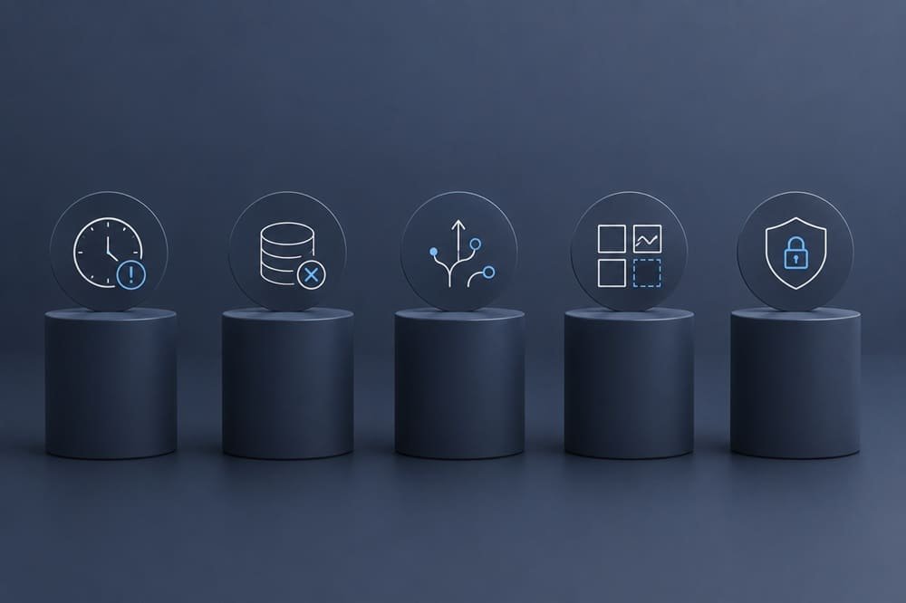
We gate every dataset that leaves DexSet through a QA pipeline built around these exact failure modes, so this post is written from the reject pile. For each of the five challenges: what it is, how it hides, how it damages training, and the check that catches it. All five checks are runnable before you spend a single GPU-hour.

Key Takeaways – The five quiet VLA training data quality failures: frame-action timestamp skew, instruction monoculture, silent failure episodes, embodiment/config drift, and mixture starvation. – Each one passes casual inspection and each one measurably degrades fine-tunes; contamination rates as low as 5-10% flatten gains on precision tasks in our ablations. – Every one has a cheap automated check; together they cost $5-9 per data-hour in our pipeline, a fraction of the GPU spend they protect. – Diversity metrics belong in acceptance criteria, not in hopes: template share, verb counts, and per-task hour caps should be contractual.

Challenge 1: Frame-Action Timestamp Skew

Timestamp skew is a systematic offset or drift between when a camera frame was captured and when the recorded action actually executed. Software timestamps on separate device clocks drift, USB cameras buffer unpredictably, and a rig that was aligned in January is often 30-50 ms off by March.

Why it hides: video looks fine, actions replay fine, and nothing is corrupt. Why it hurts: modern VLAs predict action chunks, and continuous-action heads (diffusion in Octo, arxiv.org/abs/2405.12213; flow matching in pi-zero, arxiv.org/abs/2410.24164) regress targets whose alignment with observations is the whole training signal. Skew smears that mapping. In our fine-tune ablations, loss curves separate measurably once skew passes about 10 ms, which is where we set our rig tolerance.

The fix: hardware timestamping where possible, a physical sync event at episode start (a visible gripper snap works), and an automated cross-correlation check between commanded motion and observed motion per episode. Reject on drift, do not average it away.

Challenge 2: Instruction Monoculture

Instruction monoculture is a label distribution where most episodes share a handful of sentence templates, regardless of how many total instructions exist. A 100,000-episode corpus with 14 templates is monoculture at scale; we audited exactly that situation in a recent humanoid client engagement.

Why it hides: ataset cards report episode counts, not instruction diversity – the metric that actually predicts language generalization. Why it hurts: the model learns the templates as fixed keys rather than learning language. RT-1-era templated labels produced policies with a vocabulary of about a dozen verbs (arxiv.org/abs/2212.06817); the semantic breadth in RT-2 came from web co-training, not from the robot labels (arxiv.org/abs/2307.15818). If your labels are monoculture, paraphrase failure is guaranteed.

The fix: measure template share, unique verbs, and spatial-relation coverage per batch, and set hard thresholds. We cap any single template at 8% of a batch and run paraphrase augmentation on failures. Priced honestly, a proper natural-language annotation pass adds $8-15 per data-hour. It is the least skippable line in the budget.

Challenge 3: Silent Failure Episodes

A silent failure episode is a demonstration where the task did not actually succeed – the most damaging robot dataset QA gap in teleoperation-based collection but the episode carries no failure label, so it trains the policy on a wrong outcome presented as a right one. teleoperators drop objects, miss insertions by a few millimeters, or complete the wrong variant – which is why teleoperation data collection requires explicit success criteria baked into the session protocol of an ambiguous task, and at collection pace nobody logs it.

Why it hides: failures look like successes at thumbnail resolution, and per-episode review feels too expensive so teams sample 2% and hope. Why it hurts: imitation learning has no mechanism to discount bad demonstrations; a 5-10% contamination rate is enough to visibly flatten fine-tune gains on precision tasks in our ablations.

The fix: explicit success criteria written per task family before collection, a success label as a required field, and dual review on a stratified sample weighted toward long-horizon and precision tasks. This is most of what our $5-9 per data-hour teleoperation data quality review buys.

Challenge 4: Embodiment and Configuration Drift

Configuration drift is unannounced variation in the physical setup across a collection: cameras nudged between sessions, gripper fingers swapped after wear, firmware updates that change controller latency, tables raised two centimeters. Each change is small. Accumulated, your “single embodiment” corpus is quietly five embodiments.

Why it hides: no single episode is wrong, so episode-level QA passes everything. Why it hurts: the policy either averages across configurations it cannot distinguish or keys on incidental visual cues to tell them apart. Cross-embodiment training works when variation is labeled, which is exactly how Open X-Embodiment makes 22 embodiments useful (arxiv.org/abs/2310.08864); unlabeled variation is just noise.

The fix: a per-session calibration ritual (camera extrinsics check, gripper state, controller version logged into episode metadata) and drift detection that compares session-level statistics. Metadata is free at collection time and unrecoverable afterward.

Challenge 5: Mixture Starvation

Mixture starvation is a training mixture where one data source or task family dominates sampling, starving the components that were the reason you built the mixture. It happens by accident: datasets differ in episode length, so uniform episode sampling silently overweights short-episode sources.

Why it hides: the mixture config looks balanced on paper while the effective batch composition is not. Why it hurts: OpenVLA and Octo both hand-tuned per-dataset mixture weights rather than sampling naively, and OpenVLA’s curated 970k-episode mixture is a large part of how a 7B model beat a 55B one (arxiv.org/abs/2406.09246). Teams that skip mixture sampling accounting also routinely drop web co-training too low and watch open-vocabulary grounding decay.

The fix: account mixtures in timesteps or tokens, not episodes; log effective composition per training run; cap per-task-family hours at collection time so the raw corpus starts balanced (we use a 60-hour cap per family in typical fine-tuning collections).

A note on why these five cluster together: they are all distribution problems rather than instance problems. Any single episode can pass inspection while the corpus as a whole is defective, which is why per-episode spot checks feel reassuring and prove nothing. The unit of QA for VLA data is the batch and the corpus. Once a team internalizes that, the checks below stop looking like overhead and start looking like the cheapest model improvement available.

How Do You Check VLA Training Data Quality? (5 Checks)

Challenge	Cheap Detection Check	Threshold We Use
Timestamp skew	Command-vs-observed motion cross-correlation per episode	Reject > 10 ms
Instruction monoculture	Template share + unique-verb count per 1,000-episode batch	No template > 8%
Silent failures	Success criteria + stratified dual review	5% dual-review floor
Configuration drift	Session metadata + session-statistics comparison	Any unlogged change fails
Mixture starvation	Timestep-level composition logging per run	Match declared weights ±5%

Run these against any dataset, ours included, before training on it. The full framework, including costs and the vendor RFP scorecard these checks feed into, is in the complete guide to VLA training data.

Next Step

download our free LeRobot-format sample pack and run these five checks against it yourself; the QA report ships alongside the episodes. Or start with the complete VLA training data guide.

Frequently Asked Questions

What are the most common quality problems in VLA training data?

The quiet ones: frame-action timestamp skew, instruction template monoculture, unlabeled failure episodes, unlogged configuration drift, and unbalanced training mixtures. All five pass casual inspection and all five measurably degrade fine-tunes.

How much timestamp error is acceptable in robot demonstration data?

For continuous-action models we hold frame-to-action skew under 10 ms, because our fine-tune ablations show measurable degradation beyond that. Discrete-token models tolerate more, but skew is cheap to control at capture time and expensive to fix later.

How do I check a robot dataset for label quality before training?

Measure instruction template share and unique-verb counts per batch, verify success labels on a stratified dual-reviewed sample, and cross-correlate commanded against observed motion for sync. All three checks run in hours on commodity hardware.

Why does my VLA fine-tune plateau even with more data?

Usually because the new data repeats the old distribution: same tasks, same templates, same scene. Past roughly 50-150 demonstrations per task, marginal episodes add little; audit diversity before adding volume. This is the most common symptom of undetected VLA training data quality problems in the distribution.

Case Study: How We Scaled VLA Training Data for a Humanoid Foundation Model Team

Posted on August 5, 2026July 30, 2026 by Enoch Pakanati

On station four of the collection floor, an operator sets down her leader arms after a clean bowl-to-sink transfer, and the batch dashboard flags the episode anyway. The instruction field reads “put the bowl in the sink,” the same sentence shape as two hundred episodes before it, and the template-share gate has just tripped. That flag, firing in the middle of a live program, is the single most important control in the engagement this post describes.

The client behind that program, a humanoid foundation model team, did not come to us asking for data. They came asking why their model was failing. Their OpenVLA-style fine-tune scored well on standard tabletop evaluations, then collapsed on the bimanual kitchen tasks their product actually needed. Worse, the policy only responded reliably to instructions phrased exactly like the training labels. “Put the bowl in the sink” worked. “Move that bowl into the sink” mostly did not.

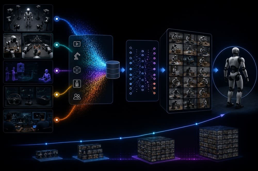
The failure had a clean explanation in their data, and it is the most common one we see. Their existing corpus was large by episode count, roughly three times what we ended up collecting, but it covered only 9 task families and used 14 instruction templates. The model had learned those 9 tasks and those 14 sentence shapes, thoroughly, and almost nothing else. Volume was never the problem. Distribution was.

This post walks through what we scoped, what the QA gates caught, what it cost in structure (with our standard benchmark rates), and what changed in their evaluations. If you are planning a fine-tuning collection, the transferable part is the method: diversity targets set as hard gates, not aspirations.

Key Takeaways – 1,400 hours of bimanual teleoperation across 42 task families replaced a corpus 3x larger in episode count but 5x narrower in tasks. – A hard instruction diversity gate (no template above 8% of any batch) fixed paraphrase brittleness; language annotation ran at our standard $12-15 per data-hour, segment-level. – Blending new data 60/40 with the legacy corpus roughly doubled held-out kitchen task success in the client’s own evaluation harness. – QA rejected 11% of collected episodes; the top three causes were teleoperator mid-chunk pauses, frame-action sync drift, and failed-but-unlabeled episodes. – Total program ran 19 weeks from scoping to final delivery in LeRobot-compatible format.

The Starting Point: A Large but Narrow Corpus

A narrow corpus is a dataset whose episode count outruns its task, scene, and language diversity, and it trains models that look strong on in-distribution tests and brittle everywhere else. The client’s legacy data was a textbook case: high volume, 9 task families, 14 templates, single kitchen scene, one camera geometry.

The published evidence already pointed to the fix. Open X-Embodiment showed pooled diversity beating single-domain volume (arxiv.org/abs/2310.08864), and Mobile ALOHA reached strong per-task results co-training with roughly 50 demonstrations per task over a broad base (arxiv.org/abs/2401.02117). Our job was to apply that at commercial fine-tuning scale on their embodiment, where cross-embodiment transfer is weakest.

What We Scoped

The collection specification is the deliverable that matters most, so we fixed it before a single episode was recorded:

Volume and spread: 1,400 robot-hours of bimanual teleoperation across 42 task families, capped at 60 hours per family to force breadth.
Scenes and objects: 6 kitchen layouts, 300+ object instances, mandated lighting variation across sessions.
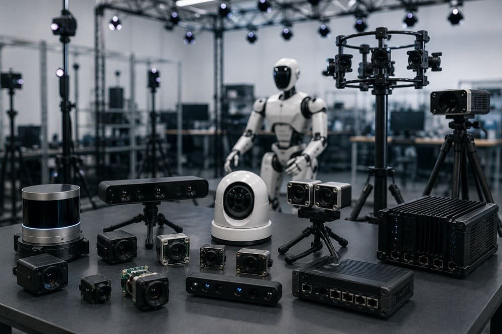
Capture spec: 4 camera streams per station (two exocentric, head, wrist), 30 Hz, hardware-timestamped, frame-to-action skew held under 10 ms.
Language spec: natural free-form instructions written at collection time, segment-level labels with timestamps on all long-horizon episodes, and the diversity gate below.
Format: LeRobot-compatible episodes so their training stack ingested data on day one (github.com/huggingface/lerobot).

The Instruction Diversity Gate

An instruction diversity gate is a batch-level QA rule that rejects any 1,000-episode batch where a single instruction template exceeds a set share, in this case 8%. Annotators drift toward comfortable phrasings; without a gate, “pick up the X and place it in the Y” quietly becomes half your labels.

We enforced three thresholds per batch: template share under 8%, minimum unique verb count, and minimum spatial-relation phrase coverage (“behind the cutting board”, “second shelf from the top”). Batches that failed went back for paraphrase augmentation before delivery. This is also where the money went: segment-level annotation with paraphrase passes ran at our standard $12-15 per data-hour, versus $8-10 for a plain episode-level pass. The client initially pushed back on that line item. It ended up being the line item their evaluation results vindicated most directly.

How the Program Ran

A collection program’s timeline is set by station-hours and reset speed, not by calendar ambition, so we planned backwards from throughput. The program ran 19 weeks across six bimanual stations: two weeks of scoping and task-family design with the client’s ML team, one week of operator training and pilot batches, fourteen weeks of production collection, and two weeks of final QA, re-collection of rejected hours, and packaging.

The pilot week matters more than its size suggests. We shipped the first 40 hours to the client immediately and they ran a smoke-test fine-tune before full production started. That surfaced two spec problems while they were still cheap to fix: their training stack expected a different gripper action convention, and one camera’s mounting height put the left workspace edge out of frame on tall-object tasks. Catching either in week twelve instead of week three would have cost hundreds of re-collected hours. If a vendor does not offer a pilot-batch gate before full-rate production, build one into the contract yourself.

Weekly deliveries went out in LeRobot format with per-batch QA reports, so the client’s dataset grew continuously instead of arriving as one end-of-program surprise.

What QA Caught

Episode rejection is the health metric of a collection program, and ours ran at 11% across the engagement. Where those episodes died:

Rejection Cause	Share of Rejects	Why It Matters for VLA Training
Teleoperator mid-chunk pauses	34%	Corrupts action-chunk targets for chunked policies (ACT-style and continuous heads)
Frame-action sync drift > 10 ms	27%	Measurably degrades continuous-action fine-tunes
Failed episode, unlabeled	22%	Success mislabeling flattens gains on precision tasks
Dropped frames / camera faults	11%	Breaks observation continuity
Instruction-episode mismatch	6%	Directly poisons language conditioning

Every rejected hour was recollected within the fixed budget because our per-hour rates ($40-60 for bimanual leader-follower work, our standard benchmark range) price in an expected rejection band. If a vendor quotes you a rate with no stated rejection policy, that risk is sitting on your side of the table.

Results

The client fine-tuned on the new corpus blended 60/40 with their legacy data and ran their internal evaluation harness before and after. Directional results, their harness, not an audited benchmark:

Held-out kitchen task success roughly doubled against the legacy-data baseline.
Paraphrased-instruction success moved from near-random to parity with template phrasing.
Long-horizon task completion improved most on tasks with segment-level labels, consistent with what the pi-zero pipeline reports about post-training data quality (arxiv.org/abs/2410.24164).

The result we quote most often is the second one, because it isolates the language layer. Nothing about the model changed. The labels changed.

What Transfers to Your Program

Four rules from this engagement apply to almost any VLA fine-tuning collection:

Audit distribution before buying volume; count task families and unique templates in your existing corpus first.
Set diversity thresholds as batch-level rejection gates, not guidelines.
Price annotation and QA as separate line items so you can see what you are cutting when you cut.
Cap hours per task family; the marginal episode of a covered task is your most overpriced purchase.

The full scoping framework, cost tables, and the RFP scorecard we build these programs from are in the complete guide to VLA training data.

Next Step

if your evaluations look like this client’s before-picture, book a scoping call. We will audit your corpus distribution before recommending a single collection hour, or start with the complete VLA training data guide.

Frequently Asked Questions

How many hours of data does it take to fine-tune a VLA for a humanoid?

This program used 1,400 hours across 42 task families, blended with existing data. Humanoids sit at the expensive end because cross-embodiment transfer from open datasets is weakest for them; standard single arms often need only 200-500 hours.

What is an instruction diversity gate?

A batch-level QA rule that rejects annotation batches where any single instruction template exceeds a set share (we used 8%), with minimum thresholds for unique verbs and spatial-relation phrases. It prevents the label monoculture that makes VLA policies brittle to paraphrasing.

Why blend new data with a legacy corpus instead of replacing it?

The legacy data still carried valid task knowledge; the 60/40 blend kept that signal while the new data corrected the distribution. Full replacement wastes paid-for coverage and can regress previously working tasks.

What rejection rate is normal in teleoperation collection?

We ran 11% on this program, and 10-15% is the band we consider healthy for bimanual long-horizon work. A vendor reporting near-zero rejection is usually not checking sync, pauses, or success labels.

5 Hidden Challenges in Data Capture Hardware for Embodied AI and How to Solve Them

Posted on July 30, 2026July 24, 2026 by Sainath Gupta

Printing your timestamps is the checklist item almost every capture team skips, and skipping it is how a ten-thousand-episode dataset dies without a symptom. We watched it happen. The dataset looked perfect: clean video, complete joint logs, delivered on time. Then the client’s policy trained to a success rate barely above random, and three weeks of forensics traced it to a 60 ms clock offset between the wrist camera and the robot controller. Every action label in the dataset was stale by two frames, and a five-line timestamp check would have caught it before the first shift ended.

Failures like this stay hidden because capture hardware fails silently, and that is the argument this post makes: silent failure is the defining property of this hardware category, so the five failure modes below must be designed out before capture, not caught after it. A camera that stops recording is obvious. A camera whose clock drifts, whose calibration decays, or whose operator quietly degrades over an eight-hour shift produces data that looks fine and trains badly. Spec sheets describe none of this, because spec sheets describe devices, not fleets running sixty-hour weeks.

This post catalogs the five failure modes my QA team catches most often, what each one costs, and the specific fix for each. All five are hardware-level problems you can design out before your first episode is recorded; the device-by-device background lives in our full guide to data capture hardware for embodied AI.

I lead data quality at DexSet, where these checks run against every egocentric, teleoperation, and multi-view batch we deliver. The thresholds below are the ones on our own QA gates.

Key Takeaways – The five hidden challenges are clock drift, calibration decay, operator fatigue, offload bandwidth, and data format lock-in. None appear on a spec sheet. – Clock drift is the most expensive: tens of milliseconds of offset silently corrupts every action label in an episode. Our QA gate rejects episodes beyond 25 ms of cross-stream misalignment. – Calibration decays with heat and handling; we re-verify extrinsics on a fixed cadence (per shift for moved rigs) rather than trusting installation-day values. – Each challenge has a cheap hardware-stage fix and an expensive post-hoc one. The table below prices both.

Challenge 1: Clock Drift and Cross-Sensor Sync

Clock drift is the gradual divergence of independent device clocks, and it corrupts the observation-action alignment that imitation learning depends on. Consumer devices drift by seconds per day; even good oscillators disagree by milliseconds per hour. A dataset can pass every visual inspection while every frame’s action label describes what the robot did 60 ms later.

The fix is architectural. Prefer hardware with a native sync story: RealSense sync pins for camera arrays, Project Aria’s shared-clock VRS recordings for wearables, robot-side timestamping for teleop streams. Where hardware sync is impossible, inject a common observable event (a strobe, an audible clap, a scripted gripper snap) at episode boundaries and align in post. Our gate rejects any episode whose residual cross-stream misalignment exceeds 25 ms.

Challenge 2: Calibration Decay

Calibration decay is the slow invalidation of a rig’s intrinsic and extrinsic parameters through heat cycles, vibration, and handling. The extrinsics you measured at installation describe a rig that no longer exists three weeks later, once a camera mount has been bumped twice and a headset has been dropped once. Depth reprojection then smears by centimeters, which is fatal for grasp-point supervision.

The fix is cadence, not heroics. We re-verify extrinsics per shift on any rig that moves (headsets, handheld UMI-style grippers) and weekly on fixed studios, using a 60-second checkerboard or AprilTag routine baked into shift startup. Rigs that fail re-verification capture nothing until they pass. The routine costs about one percent of shift time and removes our second-largest historical rejection cause.

Challenge 3: Operator Fatigue as a Data Quality Variable

Operator fatigue is the degradation of demonstration quality over a shift, and it is a hardware property as much as a human one. A 600-plus-gram headset with an external battery pack produces different data at hour six than at hour one: slower corrections, shakier trajectories, more aborted grasps. The episodes still pass automated checks. The policy trained on them inherits the sloppiness.

The fix starts at procurement. Weigh the device; anything worn for full shifts should sit near action-camera weight (~150 g) rather than headset weight (500-650 g). For teleop, seated leader-arm designs in the ALOHA style (arxiv.org/abs/2304.13705) outlast free-space VR control on repetitive tasks. Then instrument for it: we track per-operator trajectory smoothness by shift-hour, and rotate stations when the curve bends.

Challenge 4: Offload Bandwidth and Storage Starvation

Offload bandwidth is the rate at which captured data moves off devices into storage, and when it is undersized the capture floor throttles itself. A six-camera RGB-D studio generates on the order of a terabyte per shift. Teams that budget for cameras but not for the offload path end a shift early to copy files, every day, forever, and consumer devices with slow card readers make it worse.

The fix is to size the pipe with the fleet: NVMe-based ingest per capture cell, hot-swappable media so devices never wait for uploads, and compression decisions made deliberately (lossless for depth and proprioception, visually lossless for RGB) rather than by device default. As a rule we budget storage-and-offload spend at 30 to 50 percent of camera spend; audits of stalled floors usually find it under 10 percent.

Challenge 5: Data Format Lock-In

Data format lock-in is dependence on a device’s proprietary recording format, and it converts every future pipeline change into a migration project. GoPro telemetry lives in GPMF tracks, ZED records SVO files, Aria writes VRS, every teleop stack invents an HDF5 layout, and none of them agree. The cost appears later, as engineer-weeks of converters and silent unit mismatches.

The fix is to normalize at ingest, on the same day the data is captured. Pick one canonical episode schema, the LeRobot dataset format (github.com/huggingface/lerobot) is the emerging community default, and treat device-native files as transient. Keep raw originals archived, but never let a training pipeline read a vendor format directly.

How to Audit Your Own Floor This Week

A capture audit is a one-week measurement pass that scores an existing pipeline against these five failure modes, and it needs no new hardware to run. The version we use internally:

Day 1: Print timestamps. Sample 50 random episodes and compute the median camera-to-proprioception offset per episode. Anything past 25 ms goes on the findings list.
Day 2: Re-run calibration on every rig and record the delta from stored values. Deltas above your reprojection tolerance mean decay is already in your data.
Day 3: Plot per-operator trajectory smoothness by shift-hour. A visible bend after hour four is a hardware ergonomics finding, not a staffing one.
Day 4: Time one full offload cycle per cell. Any cell where offload competes with capture time loses roughly a data hour per day.
Day 5: Count the distinct file formats between device and training job. More than one canonical format plus archived originals means converter debt is accruing.

Most teams find at least three of the five on the first pass. That is not an indictment; it is the baseline this hardware category imposes on everyone.

The Five Challenges at a Glance

Challenge	Silent Symptom	Cost If Ignored	Fix at Hardware Stage	Fix After the Fact
Clock drift	Policies underperform despite clean-looking data	Entire batches rejected or retrained	Sync pins, shared clocks, boundary strobes (~$0-200/rig)	Manual event alignment; often unrecoverable
Calibration decay	Depth smears, grasp labels off by centimeters	10-20% rejection creep	Per-shift AprilTag re-verification (1% of shift time)	Re-calibration + partial batch salvage
Operator fatigue	Quality slides after hour 4	Sloppy trajectories baked into the policy	Buy light (~150 g worn), seated leader arms, rotation	Filter late-shift episodes, lose volume
Offload bandwidth	Shifts end early to copy files	~1 lost data hour/day per cell	NVMe ingest, hot-swap media (30-50% of camera spend)	Retrofit storage, disrupt operations
Format lock-in	Converter scripts multiply	Engineer-weeks per pipeline change	Normalize to one schema at ingest	Migration project across archived data

Next Step

Ready to scope your data program? Talk to our team.

Frequently Asked Questions

What is the most common hidden failure in robot data capture hardware?

Cross-sensor clock drift. Independent device clocks diverge by milliseconds per hour, silently misaligning observations and action labels. It is the failure mode least visible in review and most damaging in training.

How much clock misalignment is acceptable in a training dataset?

Our QA gates reject episodes with more than 25 ms of residual cross-stream misalignment for manipulation data. At 50-60 ms, action labels lag observations by one to two frames at 30 fps, which measurably degrades imitation learning.

How often should capture rig calibration be checked?

Per shift for any rig that moves or is worn (headsets, handheld grippers), and weekly for fixed camera studios. A 60-second AprilTag verification at shift start catches decay before it contaminates a batch.

Does operator fatigue really affect dataset quality?

Yes, measurably. On our floors, trajectory smoothness and correction latency degrade in the back half of shifts on heavy worn devices, which is why device weight and seated leader-arm ergonomics are QA concerns, not comfort perks.

What data format should robot capture pipelines standardize on?

Normalize everything to one canonical episode schema at ingest; the LeRobot dataset format is the strongest community default in 2026. Archive device-native files (GPMF, SVO, VRS) but never train from them directly.

Want these checks run for you?

Every DexSet delivery passes the five gates above before it ships. [Download Sample Data] with the QA report attached, or start with the full guide to data capture hardware for embodied AI.

5 Hidden Challenges in Teleoperation Data Collection (and How to Solve Them)

Posted on July 23, 2026July 21, 2026 by Sainath Gupta

One house rule on our collection floor reliably surprises visitors: no episode ships the day it is collected, however clean it looks on the monitor, because every episode waits for the overnight QA gate first. The rule exists because the visible challenges in teleoperation, buying rigs, hiring operators, picking a data format, are the ones teams plan for. The hidden challenges surface at episode 5,000, when the dataset is half-collected, the deadline is fixed, and the training run just exposed a flaw that has been silently poisoning every episode since week one.

That is the thesis of this post: the failures that actually kill teleoperation datasets are invisible in any single episode and only show up in aggregate, so the fix is instrumentation at ingest, not heroics at training time. Each problem looks like a minor engineering detail until it compounds. A 40-millisecond timestamp offset is invisible in a demo video. Spread across 10,000 episodes, it is the difference between a 70 percent policy and a 45 percent one.

Below are the five failures we see most often across the programs we run and audit, each with the fix we actually use. If you are new to the space, start with the complete teleoperation data collection guide and come back.

Key Takeaways – Timestamp skew between 50 Hz actions and 30 fps cameras is the top QA rejection cause we see. Gate at 33 ms, at ingest. – Operator churn is a 3x throughput event, not an HR footnote: trained operators produce 25 to 40 usable episodes per hour versus 8 to 12 for novices. – Reset drift quietly narrows your state distribution; randomization zones fix it. – QA discovered at training time is loss; QA at ingest is feedback. Expect 10 to 30 percent rejection either way, so choose when you find out. – Format decisions are nearly irreversible after 10,000 episodes. Adopt LeRobot conventions on day one.

1. Timestamp Skew: The 50 Hz vs 30 fps Trap

Timestamp skew is the misalignment between a robot’s high-rate action stream and its lower-rate camera streams, and it is the single most common reason episodes fail our QA gates. Actions log at 50 Hz; cameras deliver 30 fps; USB buffering, clock drift between machines, and software timestamps assigned at receipt rather than exposure can push streams 30 to 100 ms apart. A policy trained on skewed data learns that consequences precede actions. It will move confidently and miss.

The fix. Hardware timestamps at the sensor wherever the camera supports it; a single shared monotonic clock otherwise; and an ingest gate that rejects any episode with estimated inter-stream skew above one camera frame (33 ms). We also log a clap-style sync event at the start of each shift as a cheap ground-truth check. Action chunking in ACT-style training tolerates per-step jitter, but no algorithm recovers from systematic offset (arxiv.org/abs/2304.13705).

2. Operator Churn: The Throughput Cliff

Operator churn is the loss of trained teleoperators before their throughput has paid back their ramp cost. The ramp curve is steep: 8 to 12 usable episodes per hour in the first two weeks, 25 to 40 after certification. Every departure resets a station to novice yield for two to three weeks, which means a floor with 20 percent monthly churn is quietly running at two-thirds of its rated capacity.

The fix. Treat operators as skilled technicians, because they are. Certification gates with pay progression, per-operator quality dashboards (people improve what they can see), 45-minute session blocks on VR rigs to manage fatigue, and rig ergonomics worth caring about. Leader-follower stations retain operators better than SpaceMouse benches for the simple reason that the work feels like skill rather than struggle.

3. Reset Drift: The Shrinking State Distribution

Reset drift is the gradual narrowing of initial-state diversity as operators unconsciously converge on the fastest reset, placing objects in the same pose, episode after episode. Nobody notices because every individual episode passes QA. The policy trains beautifully, evaluates beautifully on the collection table, then fails the moment an object appears five centimeters left of its usual spot. This is how teams end up with 10,000 episodes of one initial state.

The fix. Marked randomization zones on the workspace, task cards that specify pose ranges, and a distribution monitor in the QA pipeline that plots initial object positions per task per week. When the scatter tightens, the floor lead hears about it the next morning. Datasets like DROID earned their generalization value from scene diversity, 564 scenes across 76,000 episodes, not from episode count alone (arxiv.org/abs/2403.12945).

4. Silent QA Loss: Finding Out at Training Time

Silent QA loss is the gap between episodes collected and episodes actually usable, discovered only when someone trains on the data weeks later. Rejection is not the problem; 10 to 30 percent rejection is normal and we publish those numbers. The problem is timing. Rejection found at ingest becomes operator feedback and a corrected process by tomorrow. Rejection found at training time is a hole in the dataset, a slipped deadline, and no way to know which of the last six weeks went wrong.

The fix. Nightly automated gates on every episode: sync skew, dropped frames, joint-trajectory jerk thresholds, gripper event sanity, and success-label verification against a sampled human review. Route failures to the specific operator and rig. Our floors run this as a standing morning report, and it is the highest-ROI engineering month a data program can spend.

5. Format Lock-In: The Decision You Make Once

Format lock-in is the practical irreversibility of episode schema decisions once collection is underway, because re-processing tens of thousands of episodes costs more than most teams will ever approve. Missing per-episode metadata, camera intrinsics never recorded, action spaces defined ambiguously (commanded versus measured joint positions, unlabeled): each omission is trivial to fix on day one and a migration project at episode 20,000.

The fix. Adopt community conventions before the first production episode: LeRobot dataset format for training and sharing (github.com/huggingface/lerobot), HDF5 or ROS 2 bags at capture (docs.ros.org), both commanded and measured joint states recorded, camera intrinsics and extrinsics stored per rig per calibration, and schema versioning from v0. Fifteen minutes of schema review now, or fifteen days of migration later.

How to Audit Your Own Pipeline This Week

A pipeline audit is a half-day exercise that estimates your exposure to all five hidden challenges using data you already have. No new tooling required, in most cases.

Pull ten random episodes from last month and compute the maximum camera-to-control timestamp offset per episode; anything over 33 ms means challenge one is live in your dataset right now. Ask your floor lead for usable-episodes-per-hour by operator tenure; if you cannot get the number, that absence is itself the finding. Scatter-plot initial object positions for your highest-volume task across weeks one and four of collection; visibly tightening scatter is reset drift in progress. Check when rejection is discovered: if the answer involves a training run, you have silent QA loss by definition. And finally, hand an episode file to an engineer who has never seen your schema and time how long it takes them to load actions, states, and calibrated camera streams; over thirty minutes predicts format pain at scale.

Every one of these checks has caught a live problem on programs we have audited, including our own. The five challenges are not exotic failure modes; they are the default state of a pipeline that nobody has audited yet.

The Checklist

Hidden challenge	Detection signal	Fix	Cost of ignoring
Timestamp skew	Skew estimate > 33 ms at ingest	Hardware timestamps + sync gate	Policies that act early/late; top rejection cause
Operator churn	Throughput below 20 eps/hr floor-wide	Certification, pay progression, ergonomics	Floor runs at ~2/3 capacity
Reset drift	Initial-state scatter tightening week over week	Randomization zones + distribution monitor	Policy memorizes one layout
Silent QA loss	Rejection discovered at training time	Nightly ingest gates + operator feedback	10 to 30% of budget wasted invisibly
Format lock-in	Schema questions at training time	LeRobot conventions + schema v0	Migration project at episode 20k

Next Step

Ready to scope your data program? Talk to our team.

Frequently Asked Questions

What is the most common QA failure in teleoperation data?

Inter-stream timestamp skew, typically between 50 Hz action logs and 30 fps camera streams. We gate at 33 ms of estimated skew and it remains the top rejection reason on new rigs.

How much teleoperation data fails quality checks?

Expect 20 to 30 percent rejection during the first two weeks on a new task or rig, settling to 10 to 15 percent in a mature pipeline. Budget the buffer into episode targets.

Why do teleoperation-trained policies fail on new object positions?

Usually reset drift: operators converge on repeated initial states during collection, so the dataset covers a narrow state distribution. Randomization zones and initial-state monitoring prevent it.

When should QA run on teleoperation episodes?

At ingest, nightly, never later. Rejection found at ingest becomes next-day operator feedback; rejection found at training time is unrecoverable loss weeks after the fact.

What data format should a new teleoperation program use?

LeRobot dataset conventions for training and sharing, with HDF5 or ROS 2 bags at capture. Record both commanded and measured joint states, camera calibration per rig, and version the schema from the start.

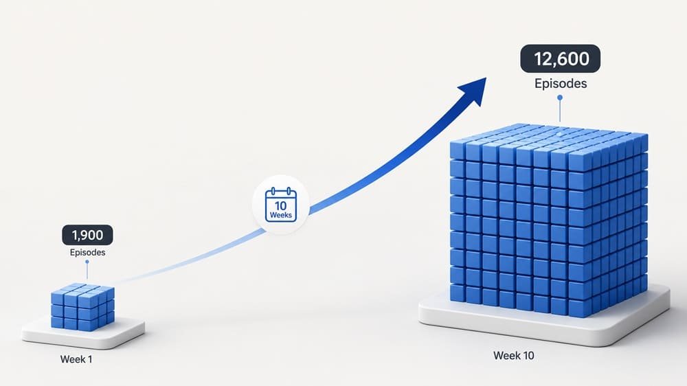
Case Study: Scaling Teleoperation Data for a VLA Model, 1,900 to 12,600 Episodes in Ten Weeks

Posted on July 22, 2026July 21, 2026 by Enoch Pakanati

A head of data once asked us which of their 1,900 collected episodes had actually made their policy better, and we could not tell them; neither could they, because nothing in their pipeline had ever connected episodes to outcomes. That question came from the team this case study is about: eight weeks into their own collection effort, 1,900 episodes against a 12,000-episode target, a 34 percent QA rejection rate, and a training deadline that had already slipped once. Their ML team was strong. Their collection operation was two engineers moonlighting as floor managers, and it showed.

This is the common failure shape, and it is the thesis of this case study. Collection stalls not because anyone lacks skill but because demonstration data is an operations problem wearing an ML costume: staffing, ergonomics, and QA gating, none of which appear in the papers. The papers do tell you what is possible; ACT hit 80 to 90 percent success from about 50 clean demos per task (arxiv.org/abs/2304.13705). Getting 12,000 clean demos across 40 tasks is a different discipline.

Here is exactly what we changed, week by week, including the two things that failed. Use it as a template for your own program, or as an argument for not running one in-house.

Key Takeaways – Baseline: 1,900 episodes in 8 weeks, 34 percent rejection. Outcome: 12,600 QA-passed episodes in 10 weeks, 12 percent final rejection. – Six leader-follower stations plus a two-week operator certification program did most of the work. – Automated ingest QA (sync skew, smoothness, completion gates) cut silent data loss to near zero. – Client’s ACT baseline improved from 41 to 68 percent average success across their internal 40-task eval. – Peak steady-state: about 1,400 usable episodes per week from 8 operators.

The Starting Point: Why 1,900 Episodes Took Eight Weeks

The client’s bottleneck was a stack of small losses, not one big one. Their audit told the story: two VR stations shared among rotating volunteers, no defined operator roles, no reset protocol, and QA performed manually by an ML engineer, at training time, weeks after collection. Rejection ran 34 percent, dominated by timestamp skew between their 50 Hz action logs and 30 fps cameras, plus inconsistent initial states that made half the “passing” episodes weak training signal anyway.

Their effective yield was under 60 usable episodes per day. At that rate the 12,000-episode target sat more than eight months out.

What We Changed

The intervention had four parts: stations, people, protocol, and gates. In order of impact:

1. Stations. We replaced the two shared VR rigs with six bimanual leader-follower stations (GELLO-class leaders on the client’s arms, roughly $300 per leader plus fabrication), keeping one VR station for the mobile-base tasks where it fit better. Joint-level control cut trajectory hesitancy immediately and shortened operator ramp.

2. People. Eight dedicated operators on a two-week certification program: task cards, reset drills, and a throughput gate (20 usable episodes per hour on a reference task) before touching production tasks. Our standard ramp curve applied; novices started at 8 to 12 usable episodes per hour and certified operators stabilized at 25 to 40.

3. Protocol. Written task cards for all 40 tasks, marked randomization zones for object placement, success criteria defined at collection time, and per-episode metadata (task, operator, rig, success) attached at the source.

4. Gates. Automated ingest QA running nightly: inter-stream sync skew over 33 ms flagged, dropped-frame counts, jerk thresholds on joint trajectories, and completion labels verified against a sampled human review. Failures routed back to the floor as next-morning feedback per operator, which mattered as much as the gate itself.

The Week-by-Week Numbers

Weekly usable output tells the ramp story better than any narrative.

Week	Usable episodes	Rejection rate	Notes
1	310	29%	Station bring-up; operators in certification
2	540	26%	First cohort certified; jig redesign after reset failures
3	980	19%	All 8 operators on production tasks
4	1,390	15%	Steady state reached
5 to 9	1,300 to 1,450/wk	11 to 14%	Two task cards rewritten after eval feedback
10	1,280	12%	Target passed: 12,600 total QA-passed

Two failures worth admitting. In week two, our first reset jig for a deformable-object task increased reset time instead of cutting it; operators beat the jig by hand and we scrapped it. And one of the 40 tasks, bimanual jar opening, ran a stubborn 25 percent rejection until week six, when slowing the commanded demonstration pace fixed what better hardware had not.

Did the Data Actually Help? Policy Results

The point of episode counts is policy performance, so the client re-trained their ACT baseline on the new corpus at week eleven. Average success across their internal 40-task evaluation went from 41 percent (trained on their original 1,900 mixed-quality episodes) to 68 percent, with the largest gains on precision tasks where the old VR data had been noisiest. Same architecture, same hyperparameter budget, different data. Their team’s summary, which we will keep quoting: “We spent six months on model changes for less improvement than ten weeks of better data.”

That is one program, not a controlled study, and we flag it as such. But it matches the pattern across our floors and the published record: demonstration quality moves policy success more reliably than architecture iteration at this stage of the field.

What We Would Do Differently

Every program teaches something, and this one taught us three corrections we have since made standard. First, we would start the operator certification cohort a full week before station bring-up finishes, not after. Waiting for hardware serialized two ramps that could have run in parallel, and it cost the program most of week one’s output. Second, we would pilot every task card ourselves before handing it to operators. Two of the 40 cards contained ambiguous success criteria (“lid secured” without a torque or rotation definition), and the resulting label inconsistency did not surface until the week-five training run flagged suspicious loss on exactly those tasks. A ten-minute pilot per card would have caught both. Third, we would set the deformable-object tasks to a slower commanded pace from day one. The week-six discovery that pace, not hardware, drove the jar-opening rejection rate had been sitting in the per-task rejection data since week two; we were looking at floor-level averages and missed it. Per-task dashboards are now default on every program we run.

None of these are exotic lessons. That is rather the point: scaling demonstration data is a discipline of small, boring corrections applied early, and the gap between 1,900 episodes and 12,600 episodes was made of exactly such corrections.

The Reusable Checklist

Scaling teleoperation collection comes down to seven decisions made early:

Match rig to task family (leader-follower for fine bimanual work; VR for mobile/humanoid tasks)
Dedicated, certified operators, never rotating volunteers
A throughput gate before production collection
Written task cards with randomization zones and success criteria
Hardware timestamps on every stream; sync checked at ingest, not at training
Nightly automated QA with per-operator feedback loops
A rejection buffer of at least 15 percent in the episode target

Rig options, cost-per-episode math, and QA thresholds are covered in depth in the complete teleoperation data collection guide.

Next Step

Ready to scope your data program? Talk to our team.

Frequently Asked Questions

How many episodes does a VLA model program need?

Program-dependent, but the humanoid teams we support typically target 10,000 to 50,000 QA-passed episodes per quarter across dozens of tasks. Single-task ACT policies can work from about 50 clean demos; multi-task generalization is what drives volume.

How long does it take to scale a teleoperation data program?

With rigs, certified operators, and ingest QA in place, expect three to four weeks to steady state. This program reached about 1,400 usable episodes per week from 8 operators by week four.

What rejection rate should I budget for?

At least 15 percent at maturity and 25 to 30 percent during the first two weeks of any new task or rig. Budgeting zero rejection is the most common planning error we see.

Is it cheaper to collect teleoperation data in-house or outsource it?

In-house costs more than teams expect once engineer time is counted; the client here spent eight engineer-weeks producing data that mostly failed QA. Outsourcing wins on time-to-data in most cases; in-house wins when collection is itself a core competency you intend to build.

What improved policy success most in this case study?

Rig fidelity and QA gating together. Joint-level leader-follower control removed trajectory hesitancy, and ingest gates stopped skewed episodes from reaching training. Success rose from 41 to 68 percent with no model changes.

Case Study: How a Series B Humanoid Startup Rebuilt Data Procurement for Its VLA Model

Posted on July 14, 2026July 16, 2026 by Enoch Pakanati

Grasp success on the team’s fixed eval suite dropped six points in a single week, and for two days nobody could explain it. The model had not changed. The training code had not changed. What had changed, it eventually emerged, was a data batch: one of their three vendors had silently rescaled gripper actions between deliveries. The team had money, talent, and a working humanoid platform. What stalled their VLA program was procurement: three data vendors, three delivery formats, no shared acceptance spec, and an ML team that had quietly stopped trusting incoming data. By their own estimate, roughly a quarter of purchased hours never reached a training run.

Nothing about that situation was unusual. It is what happens when data purchasing grows by accretion: a vendor added for a demo push here, another for a task category there, each with its own definitions of “hour,” “annotated,” and “calibrated.” The result is not one data pipeline but several, with the training team as the manual integration layer.

This post walks through how the team rebuilt procurement in one quarter using the four artifacts from the Robotics Data Buyer’s Playbook: a spec-first RFP, a weighted scorecard, a red flags screen, and a 50-hour paid pilot. The client is anonymized (a Series B humanoid startup; we do not name customers), but the process and the numbers are the real pattern we see when buyers switch from improvisation to protocol. The thesis this case argues: pilots run under production conditions predict production performance, and paper evaluation alone does not.

DexSet was one of the vendors evaluated in this process, so we saw the RFP, the pilot, and the contract from the receiving side. That is exactly the vantage point a buyer should want documented.

Key Takeaways

Starting point: three vendors, three formats, ~74 percent average usable-hour yield, about one engineer-day of triage per delivery.
The rebuild: one written acceptance spec, an RFP to six vendors, a 10-criterion weighted scorecard, paid 50-hour pilots for the top two.
Pilot results diverged sharply: 90 percent yield with a positive policy delta versus 78 percent yield and a failed loader test.
Twelve weeks later: yield held within two points of the pilot across the first 1,000 contracted hours, and per-delivery engineering time dropped from a day to under an hour.

The Starting Point: Accretion, Not Architecture

The team’s data supply had accreted rather than been designed: each vendor relationship was created for a short-term need, and none was ever re-evaluated. Vendor A delivered undocumented HDF5 with a schema that shifted between batches. Vendor B delivered rosbag2 that had to be converted and re-timestamped. Vendor C delivered mp4s plus CSV joint logs with no sync guarantees at all.

The measurable symptoms, from their own tracking:

Average usable-hour yield around 74 percent across vendors, measured against the acceptance checks they eventually wrote down.
Roughly one engineer-day per delivery spent on conversion and triage.
Two training regressions in one quarter traced back to data batches, one to a sync drift issue, one to inconsistent gripper action scaling between vendors.

The trigger for change was mundane: a planning meeting where nobody could answer what an incremental 1,000 hours of manipulation data would actually cost, because nobody could say what fraction would be usable.

Step 1: Write the Spec Before Talking to Anyone

The acceptance spec is a short document that defines what a usable hour means for a specific program, and writing it was the most valuable week of the whole rebuild. Theirs fit on three pages: stereo egocentric plus wrist cameras at defined resolutions and frame rates, proprioception at 50 Hz minimum, time sync under 10 ms across all streams, a 60-task manipulation list with reset criteria, an annotation rubric, and delivery in LeRobot format with a schema doc, following the conventions the ecosystem inherited from Open X-Embodiment and the ALOHA line of work (arxiv.org/abs/2310.08864; arxiv.org/abs/2304.13705).

The immediate effect was that vendor quotes became comparable for the first time. The secondary effect was internal: the ML and data teams had to agree on what they were actually buying, which surfaced two silent disagreements about camera placement that had been corrupting cross-vendor consistency for months.

Step 2: RFP and Scorecard

The RFP went to six vendors with fifteen questions requiring numeric answers: committed usable-hour yield, sync tolerance and recheck cadence, audit accuracy, rig counts behind throughput claims, per-hour pricing by task complexity, pilot terms, and licensing. Four vendors answered with numbers. Two answered with adjectives and were dropped without further calls, which is the red flags screen doing its job cheaply.

The four remaining responses were scored independently by two people on the 10-criterion weighted scorecard (quality SLAs 15, modality coverage 12, calibration/sync 12, down to IP/licensing at 7). Independent scoring earned its keep in the reconciliation meeting: the two scorers disagreed by more than a point on only three criteria, and every disagreement traced to an ambiguous vendor answer rather than a difference in judgment. Those ambiguities went back to the vendors as written clarification requests, which is a politer and more useful outcome than one person’s optimism deciding the ranking.

The scoring separated the field more on contract terms than on hardware: two vendors wanted broad rights to reuse delivered episodes for other customers, which the team treated as disqualifying on the licensing criterion. Two finalists advanced.

Step 3: The 50-Hour Paid Pilots

Both finalists ran paid 50-hour pilots under production conditions, judged on four numbers fixed in the pilot agreements before capture began. This is the step that paper evaluation cannot replace, and the results diverged more than the scorecards had predicted.

Pilot metric (agreed in advance)	Threshold	Finalist 1	Finalist 2
Usable-hour yield vs acceptance spec	≥85%	90%	78%
Annotation accuracy (independent 5% re-label)	≥97%	98.2%	96.1%
Policy success delta on fixed 12-task eval	Positive	+6 points vs baseline	+1 point
Loader time into LeRobot pipeline	≤1 engineer-day	~2 hours	Failed (schema mismatches, 3+ days)

The policy-delta test deserves a note. The team fine-tuned the same fixed baseline policy twice, once on their existing mix, once with the 50 pilot hours added, and evaluated both on the same 12 tasks. Fifty hours is a small delta at VLA scale, and they treated it that way: not as proof of final performance, but as a canary. Data that helps at 50 hours might help at 1,000; data that does nothing at 50 hours is a warning you can act on before signing an annual contract.

Step 4: Contract and the Twelve Weeks After

The contract encoded the pilot numbers rather than replacing them with prose: yield commitment at 88 percent with redelivery of failures, sync tolerance and recalibration cadence as delivery requirements, LeRobot schema versioned in an appendix, quarterly re-audit rights, and no vendor reuse of delivered episodes.

The results over the first 1,000 contracted hours were unremarkable in the best sense. Yield held between 88 and 90 percent, within two points of the pilot. Engineering time per delivery fell from roughly a day to under an hour, because the format and schema were locked before signature instead of negotiated after each batch. The two silent disagreements about camera placement did not recur, because the spec, not tribal memory, was the reference.

The honest caveat: this process cost about five weeks end to end and roughly $7,000 in pilot fees across two finalists. For a team spending six figures annually on data, that insurance premium was around 5 percent of program cost. For a team buying 20 exploratory hours, it would be overkill, and we say so in the full playbook.

Next Step

Ready to scope your data program? Talk to our team.

Frequently Asked Questions

How much did the procurement rebuild cost compared to what it saved?

About five weeks of process time and roughly $7,000 in paid pilot fees. Against it: yield moved from ~74 to ~90 percent, and per-delivery engineering time dropped from a day to under an hour, which on a six-figure annual program repaid the process cost within the first deliveries.

Why run paid pilots with two finalists instead of one?

Because scorecards rank paper, and paper can lie by omission. In this case the two finalists scored within a few points of each other, then diverged by 12 yield points and a failed loader test under production conditions.

Is a 50-hour pilot enough to judge data for a VLA model?

It is enough to judge the vendor’s pipeline, not the model’s ceiling. Treat the policy success delta as a canary: positive movement at 50 hours justifies scaling; zero movement is a cheap warning.

What belongs in the contract that most teams leave out?

The pilot numbers themselves: yield commitment with redelivery terms, sync tolerance as a delivery requirement, a versioned schema appendix, re-audit rights, and an explicit ban on vendor reuse of delivered episodes.

5 Hidden Challenges in Exocentric & Multi-View Data for Robot Learning (and How to Solve Them)

Posted on July 1, 2026July 16, 2026 by Sainath Gupta

Multi-view data is usually defined as episodes recorded from several calibrated, synchronized cameras. That definition hides the real problem: calibration and synchronization are not properties you establish, they are properties you maintain, and every mechanism that breaks them is invisible on the day it happens. A dead camera stops a capture session; everyone notices, everyone fixes it. A tripod nudged 4 millimeters by a cleaning crew stops nothing. Capture continues for three weeks, the extrinsics in the metadata quietly stop matching reality, and the first symptom appears a month later as a training curve that will not converge, in a building the data team does not work in.

That gap between when multi-view data breaks and when anyone finds out is what makes these challenges “hidden,” and it is the thesis of this post: detection latency, not defect rate, is what actually determines the cost of a multi-view failure. Single-view pipelines fail loudly. Multi-view pipelines add cross-camera dependencies (shared clocks, relative poses, matched exposure) that fail silently, and the cost of the failure scales with how long it goes undetected.

I run data quality at DexSet, which means my job is finding these failures before customers do. This post covers the five that account for nearly every multi-view escalation we have handled, each with the fix we actually use, not the fix that sounds good in a slide. Rig geometry, camera selection, and cost context live in the pillar: The Complete Guide to Exocentric & Multi-View Data for Robot Learning.

Key Takeaways – The five silent killers: calibration drift, time sync skew, storage blowup, viewpoint overfitting, and lost extrinsics metadata. – Every fix is procedural, not exotic: per-session verification sweeps, PTP or hardware triggering, codec decisions before capture, view dropout in training, and extrinsics embedded per episode. – Our gates: reprojection error under 0.5 px and cross-camera skew under 10 ms, checked every session. Sessions that fail do not ship. – Detection latency is the real enemy. A defect caught same-day costs minutes; caught post-training, it costs a recollection.

Challenge 1: Calibration Drift

Calibration drift is the gradual or sudden divergence between a rig’s recorded extrinsics and its physical camera poses, caused by bumped mounts, sagging booms, thermal cycles, or fixture swaps. It is the most common defect we see in incoming third-party datasets, and the most expensive, because every frame captured after the drift event carries wrong geometry.

The failed solution is calibrating on install and trusting the mounts. Mounts do not deserve trust. Our fix has three parts: rigid fixturing over convenient fixturing (no friction-arm boom mounts on anything that ships), a 20-second ChArUco verification sweep at the start of every session, and a hard ingestion gate at 0.5 px reprojection error. The sweep costs two minutes. In one recent engagement it caught a sagged mount at 1.3 px the morning after a fixture swap; 25 minutes of recalibration instead of weeks of poisoned data. The toolchain is standard: OpenCV calibration for intrinsics and stereo pairs, Kalibr for full multi-camera rigs, ROS 2 camera_calibration for live-topic workflows.

Challenge 2: Time Synchronization Skew

Sync skew is disagreement between cameras about when a frame was captured, and it turns multi-view supervision into contradiction: two views of “the same instant” showing the gripper in two different places. At 30 fps, a one-frame offset is 33 ms of world-state disagreement, injected into every training sample, unremovable after the fact.

Software timestamps drift because independent device clocks drift; that is not a bug, it is physics. The fix is choosing a sync tier deliberately. PTP (IEEE 1588) disciplines clocks over Ethernet to sub-millisecond agreement and is the right default for GigE cameras. Hardware trigger lines or genlock drive shutters from one signal and are mandatory for fast motion. Consumer RGB-D units vary: the RealSense D455 exposes a sync pin, the OAK-D accepts GPIO triggering, the ZED 2i relies on timestamps. Two operational rules: put every sensor on the same clock domain, including wrist cameras running off arm controllers (we once shipped a pilot with an 18 ms wrist offset from exactly that mistake), and verify skew every session against a shared event, gated at 10 ms for manipulation work.

Challenge 3: Storage and Throughput Blowup

The storage blowup is the 3x to 4x multiplication of data volume that multi-view imposes on every downstream system: disks, network links, ingestion jobs, QA review time, and cloud egress bills. A 4-camera rig at 1080p30 produces 0.8 to 1.5 TB per capture day in our pipelines. Teams that budgeted storage for single-view discover this at the worst possible moment, mid-program.

The fix is making format decisions before the first capture day. Choose the codec deliberately (we deliver H.265 for RGB streams; raw or lightly compressed depth where the training plan needs it), define retention tiers so raw footage does not live on hot storage forever, and, most importantly, decide camera count with an ablation instead of ambition. DROID shipped roughly 76,000 episodes with three views, not eight (arXiv:2403.12945); in our own ablations the fourth camera adds about 25 percent to storage and QA cost while rarely moving policy success.

Challenge 4: Viewpoint Overfitting

Viewpoint overfitting is a policy’s silent dependence on the exact camera poses it was trained with, so that a deployment camera mounted 10 cm off the training pose degrades performance without any visible domain shift. It is the mirror image of the problem multi-view was supposed to solve, and fixed rigs make it worse: perfectly consistent extrinsics are perfectly consistent spurious features.

The solution operates on both sides of the pipeline. On capture: introduce controlled pose variation across stations and sessions (a few degrees and centimeters, logged in the extrinsics, never random and unrecorded). On training: view dropout and view shuffling, so the model cannot rely on any single camera being present, a practice consistent with RoboMimic’s finding that observation space composition materially shifts outcomes (arXiv:2108.03298). Ego-Exo4D’s paired design (arXiv:2311.18259) shows the research-grade version: cross-view correspondence learned explicitly rather than avoided.

Challenge 5: Lost Extrinsics and Metadata Decay

Metadata decay is the separation of calibration and sync records from the episodes they describe, until the dataset becomes multi-view footage with no usable geometry. The classic form: extrinsics live in a wiki page or a calib_final_v3.yaml on someone’s laptop, the rig changes, the file does not, and two years later nobody can say which episodes match which calibration. Much of the viewpoint friction in aggregated corpora like Open X-Embodiment (arXiv:2310.08864) traces back to exactly this: heterogeneous sources where camera geometry was never packaged with the data.

The fix is structural: embed per-camera intrinsics, extrinsics, sync offsets, and the calibration verification result inside every episode’s metadata, written by the capture software, not by a human. An episode should be self-describing forever. We also version calibrations with timestamps and station IDs, so any historical episode can be traced to the exact calibration event that produced its geometry.

The Five Challenges at a Glance

Challenge	Silent Symptom	Fix	Our Gate
Calibration drift	Training noise weeks later	Per-session ChArUco sweep, rigid mounts	< 0.5 px reprojection error
Sync skew	Cross-view label contradiction	PTP / hardware trigger, shared clock domain	< 10 ms cross-camera skew
Storage blowup	Budget collapse mid-program	Codec + retention decided pre-capture; ablate camera count	~1 TB/day per 4-cam rig planned
Viewpoint overfitting	Deployment-time degradation	Logged pose variation + view dropout in training	Pose deltas recorded per session
Metadata decay	Unusable geometry years later	Extrinsics embedded per episode, versioned	Episode self-describing, machine-written

Audit Your Rig Before It Audits You

Every one of these five failures has a one-line question that exposes it in a vendor conversation, and we have collected them into the Multi-View Rig RFP Scorecard. Download it before your next data procurement call, or use it to audit your own rig. Either way, ask the reprojection error question first.

Frequently Asked Questions

What is the most common failure in multi-view robot datasets?

Calibration drift: physical camera poses diverging from recorded extrinsics after bumps, sag, or fixture changes. It is silent at capture time and surfaces later as training noise, which is why per-session verification with a reprojection error gate is the standard fix.

How much sync error is acceptable between cameras?

For tabletop manipulation at 30 fps, DexSet gates at 10 ms cross-camera skew; a full frame of offset (33 ms) injects visible world-state contradiction into training pairs. Fast or dynamic tasks need hardware triggering rather than timestamp alignment.

How do I stop a policy from overfitting to camera positions?

Combine controlled, logged pose variation across capture sessions with view dropout during training, so the model cannot depend on any exact camera pose or on every view being present.

How much storage does multi-view capture need?

Plan for 3x to 4x your single-view volume: roughly 0.8 to 1.5 TB per capture day for a 4-camera 1080p30 rig with H.265 RGB, more if depth streams are kept raw. Decide codecs and retention tiers before capture begins.

Where should calibration data be stored?

Inside every episode’s metadata, written automatically by the capture software: per-camera intrinsics, extrinsics, sync offsets, and the session’s verification result. External calibration files decay; self-describing episodes do not.

Case Study: How We Scaled Exocentric & Multi-View Data for a VLA Model

Posted on June 30, 2026July 16, 2026 by Enoch Pakanati

We once shipped a pilot batch with an 18 millisecond wrist-camera clock offset, and this case study exists partly because of it. The mistake was ours: the wrist stream was timestamped off the arm controller instead of the rig’s PTP clock domain, invisible in playback, and it was the customer’s smoke-test training run at hour 20 that surfaced it. We fixed it, changed our rig standard, and kept the lesson. Vendor case studies that report zero mistakes are describing a project that never touched hardware.

This one covers eight weeks of work with a humanoid foundation model team (anonymized by agreement) whose manipulation policy had stalled on cluttered-scene tasks. The claim we will argue with the numbers below: their ceiling was informational, not architectural, and a disciplined multi-view capture operation, pilot batches, per-session calibration gates, one shared clock domain, is what removed it.

The team arrived with a specific complaint. Their policy trained fine, evaluated fine on open scenes, then dropped hard on cluttered tabletops. Their dataset: tens of thousands of teleoperated episodes, every one recorded from a single fixed camera. Failure review showed what you would expect. When clutter occluded the target from that one viewpoint during approach, the policy guessed.

They asked us for multi-view capture at a rate their internal rig could not hit: hundreds of hours within a quarter, calibrated, synchronized, and QA’d to a standard their ML leads could defend. What follows is how we built it, what it cost, what broke, and what the retrain showed. For the general framework behind these choices, the pillar guide is here: The Complete Guide to Exocentric & Multi-View Data for Robot Learning.

Key Takeaways – 600 hours of DROID-style multi-view episodes (two external stereo + wrist) delivered across 8 weeks on 4 parallel stations. – Per-session calibration gates rejected 4.1 percent of sessions; every rejection would have shipped corrupted extrinsics without the gate. – All-in capture cost landed at $31 per hour, inside our standard $26 to $38 benchmark range. – Retrained on matched episode counts, the customer’s occlusion-heavy split improved by double digits; open-scene performance held.

The Starting Point: Diagnosing a Data Ceiling

A data ceiling is a performance plateau caused by information missing from the training set rather than by model capacity. Confirming one is cheap and worth doing before any capture contract: tag evaluation failures by whether the target object was visible to the training viewpoint at decision time. On this team’s cluttered-scene split, occlusion-correlated failures dominated by a wide margin. No architecture sweep fixes pixels that were never captured.

The finding matches the public record. The RoboMimic study showed observation space design materially changes imitation outcomes on identical demonstrations (arXiv:2108.03298), and DROID’s authors considered multi-view important enough to mandate two calibrated external stereo views plus wrist across all 76,000 episodes (arXiv:2403.12945). We proposed the same geometry rather than inventing one.

The Rig Spec: Boring by Design

The capture spec is the contract between operations and the ML team, and ours fit on one page. Four identical stations, each with:

Two ZED 2i stereo cameras on rigid tripod mounts at roughly 45 degrees off the workspace centerline, 1 m from task center, opposite sides.
One wrist camera on the arm.
Extrinsics calibrated with a ChArUco target via OpenCV, cross-checked in Kalibr; camera-to-robot-base transform verified against known end-effector poses.
Sync via PTP-disciplined clocks, with a hard gate: cross-camera skew under 10 ms or the session does not ship.
A 20-second ChArUco verification sweep at every session start; reprojection error above 0.5 px blocks capture until recalibration.

Identical stations mattered more than any individual choice. One geometry means one calibration procedure, one QA script, one training data schema, and operators who can rotate between stations without retraining.

What Eight Weeks Actually Looked Like

Scaling capture is a throughput problem with a quality constraint, and the numbers tell the story better than prose:

Metric	Value
Capture stations	4 (identical DROID-style geometry)
Calendar time	8 weeks
Delivered episodes	~58,000 across 41 task variants
Delivered hours (multi-view)	600
Sessions rejected at calibration/sync gate	4.1%
Episodes rejected at QA review	2.7%
Storage delivered	~38 TB (H.265, with per-frame extrinsics and sync metadata)
All-in operated cost	$31 / hr

Weeks one and two ran at half throughput on purpose. We shipped a 20-hour pilot batch first so the customer’s ML team could confirm schema, load episodes into their LeRobot-based training stack, and run a smoke-test train before we committed the fleet. They caught the wrist-camera clock defect described at the top of this post: a consistent 18 ms offset from timestamping off the arm controller instead of the PTP domain. Catching that at hour 20 instead of hour 600 is the entire argument for pilot batches.

Throughput past the pilot came down to two decisions that had nothing to do with cameras. The first was task design: the customer’s 41 task variants were sequenced so that each station ran one object set per half-day block, which cut resets and scene changes to minutes instead of the constant churn you get when operators bounce between tasks. The second was operator rotation. Because all four stations shared one geometry and one procedure, any operator could run any station, and we scheduled captures to keep stations busy through breaks and calibration stops. Utilization across the fleet held near 85 percent of scheduled hours; on prior projects with heterogeneous rigs, we had struggled to hold 65.

The other failure worth naming: in week five, a boom mount on station three sagged after a fixture swap, and the morning verification sweep caught reprojection error at 1.3 px. The gate rejected the session, recalibration took 25 minutes, and no corrupted data shipped. Before we ran per-session gates, that class of drift used to surface weeks later as unexplainable training noise.

The Result: What the Retrain Showed

The customer retrained the same architecture on matched episode counts, single-view versus our multi-view data, which is the only comparison that isolates the data effect. On their occlusion-heavy cluttered split, success improved by double digits. On open scenes, performance held flat, confirming the ceiling had been informational, not architectural. Their engineers also reported a second-order win: with three calibrated views per episode, failure triage became visual inspection instead of guesswork, because someone could always see what happened.

We report ranges rather than their exact internal metrics by agreement, and we would flag any vendor who publishes a client’s precise evaluation numbers as a reason to negotiate confidentiality carefully. What we can say precisely is what the comparison controlled for: same architecture, same hyperparameters, same episode count, same evaluation protocol. The only variable was the data.

What We Would Repeat, and What We Changed

Three practices carried the project and are now standard on every DexSet engagement: pilot batches before fleet commitment, per-session calibration and sync gates with hard thresholds, and extrinsics embedded in every episode’s metadata rather than in a side document that drifts out of date.

One thing we changed afterward: we now put the wrist camera on the PTP domain from day zero, on every rig, because the 18 ms lesson generalizes. And we stopped quoting capture programs without a failure-tagging pass on the customer’s existing evaluation data first; twice since, that pass showed the bottleneck was not viewpoint at all, and we said so.

Test the Pattern on Your Own Failures

If your evaluation failures cluster around occlusion and your dataset is single-view, the pattern in this case study probably applies to you. Book a demo and we will walk through the pipeline with real sample episodes, calibration metadata included, and run the failure-tagging pass on your evaluation data before anyone talks about a contract.

Frequently Asked Questions

How long does it take to scale a multi-view capture program?

In this engagement, 600 hours of calibrated multi-view data took 8 weeks on 4 parallel stations, including a deliberately slow 2-week pilot phase. Throughput scales roughly linearly with identical stations once the geometry and QA gates are standardized.

What did the multi-view data cost?

All-in operated capture landed at $31 per hour, inside DexSet’s standard $26 to $38 benchmark range for DROID-style rigs, plus one-time rig builds in the $4,500 to $7,000 range per station.

How do you verify calibration at scale?

A 20-second ChArUco verification sweep at every session start, gated on reprojection error under 0.5 px, with extrinsics cross-checked in Kalibr and camera-to-base transforms verified against known end-effector poses. Sessions failing the gate are recalibrated before any capture ships.

Did multi-view data actually improve the VLA policy?

Yes. Retrained on matched episode counts, the customer’s occlusion-heavy evaluation split improved by double digits while open-scene performance held, isolating viewpoint coverage as the binding constraint.

Why run a pilot batch before full capture?

Because schema and sync defects are cheap at hour 20 and expensive at hour 600. The pilot here caught a wrist-camera clock offset of 18 ms that would otherwise have contaminated the full delivery.

5 Hidden Challenges in Egocentric Data Collection for Robotics and How to Solve Them

Posted on June 29, 2026July 16, 2026 by Enoch Pakanati

Aviation stopped losing aircraft to dramatic causes decades ago; what remained were the quiet ones, a skipped checklist item, an ambiguous callout, a gauge that read normal until the moment it mattered, and the industry’s answer was to treat small procedural failures as the primary safety problem rather than a footnote. Egocentric data collection is living through the pre-checklist era of that same history. Budgets and rig choice get argued about in every kickoff meeting, so they get managed. The hours that actually get rejected in my QA queue fail for quieter reasons: a timestamp that drifted 80 milliseconds, an auto-exposure loop hunting under warehouse LEDs, a bystander’s face where a consent form should be.

These failures stay hidden because each one is invisible at capture time. The collector sees a normal recording. The file uploads fine. The problem surfaces weeks later, when an engineer tries to align IMU packets with video frames, or a lawyer asks who signed off on the person in frame 40,000. By then the collection trip is over and the fix is a re-shoot. That is this post’s thesis: the failures that destroy egocentric datasets are procedural and invisible at capture time, so only enforced process, not better hardware, catches them before they compound.

I review egocentric footage for a living, roughly a few thousand hours a quarter across DexSet’s programs. This post covers the five failure modes that cost our clients (and, in the early days, us) the most money, what each one does to your training data, and the fix we now enforce by default. Every one of these is checkable before you scale, and none of them appears on a hardware spec sheet.

Key Takeaways – The expensive failures in egocentric collection are invisible at capture time: sync drift, exposure instability, bystander privacy, protocol drift, and metadata chaos. – Sensor sync should be verified per session, not trusted; drift beyond ~10 ms between IMU and frames degrades ego-motion estimation and any action retargeting built on it. – Auto-exposure and rolling shutter quietly poison fast-motion segments; lock exposure ranges per environment and test at task speed. – Privacy is a data-quality gate, not just a legal one; footage you cannot license cleanly is footage you cannot ship, whatever its pixel quality. – Fixing these adds roughly $2 to $5 per hour in process cost and saves multiples of that in rejected hours; our first-pass yields moved from ~70 to 85+ percent after enforcing the five fixes below.

Challenge 1: Sensor Sync Drift

Sensor sync drift is the accumulating misalignment between timestamps of different streams (video frames, IMU packets, depth, gaze) recorded on the same rig. Consumer devices are the usual culprits: separate clocks, buffered writes, and dropped packets each add error, and error compounds over a 40-minute session.

Why it hurts: ego-motion estimation fuses IMU with frames, and hand-trajectory extraction inherits any misalignment as velocity noise. Once drift passes roughly 10 ms, we see it in reprojection error; past 30 ms, retargeting-grade annotation is off the table for that session. Purpose-built devices earn their price here; Aria-class glasses timestamp all streams against a common clock with factory calibration (projectaria.com), which is a large part of why their finished-hour costs are competitive despite the hardware premium.

The fix: a physical sync event at every session start and end (a clap or strobe visible to all sensors), automated drift measurement between the two events, and a hard QA gate. On custom RealSense rigs, we also pin capture to hardware timestamps rather than host arrival times. Cost: seconds per session and one script.

Challenge 2: Auto-Exposure and Motion Blur at Task Speed

Auto-exposure instability is the camera’s exposure control oscillating or lagging as the wearer’s head sweeps between bright and dark regions, and it is the single largest source of rejected kitchen and warehouse footage in our logs. Head-mounted cameras experience scene luminance changes far faster than handheld ones. Add rolling shutter and fast hand motion and you get smeared, flickering segments exactly where the manipulation happens.

The insidious part is that slow test recordings look fine. Collectors validate the rig while standing still; the failure only appears at task speed, and encoders trained on smeared hands learn smeared hands.

The fix: per-environment exposure presets (shutter-priority for fast tasks), a five-minute test capture at full task speed before every new location, and an automated blur metric in the QA pipeline. On GoPro-class rigs we run higher frame rates (60 to 120 fps) to buy shutter headroom. This one protocol change moved a client program’s first-pass yield by eight points.

Challenge 3: Bystander Privacy and Consent

Bystander capture is the recording of people who never consented to be in your dataset, and in egocentric collection it is the default outcome rather than the exception, because the camera goes wherever the collector’s head turns. Large academic efforts treated this as a first-class problem; Ego4D built consent processes and de-identification into its collection across 74 locations (arXiv:2110.07058), and commercial programs are held to a stricter standard, not a looser one.

Treat this as data quality, not legal overhead: an hour you cannot license is an hour you cannot deliver, and face-blurring after the fact degrades exactly the frames where a person interacts with the scene.

The fix: controlled capture sites with posted notice and signed consent for everyone who could enter frame, collector training to pause on unexpected entries, and automated face/plate detection as a QA flag rather than a silent blur. Where blurring is unavoidable, we log it in episode metadata so downstream users can filter.

Challenge 4: Protocol Drift Across Collectors and Weeks

Protocol drift is the slow divergence between what your task specification says and what collectors actually do by week six. Human demonstrators optimize for their own comfort: grasps migrate to five-finger tricks a parallel-jaw gripper cannot copy, “reset the scene” becomes approximate, and each site develops a local dialect of the task. None of this looks like an error in any single episode. In aggregate, it shifts your action distribution away from anything a robot can imitate, widening the embodiment gap that retargeting work like EgoMimic goes to such lengths to close (arXiv:2410.24221).

The fix: written task cards with start-state photos and outcome rules, motion constraints stated in robot terms (gripper envelope, reach profile), weekly sampled review per collector rather than per batch, and re-training triggered by drift metrics instead of complaints. Episode-structured schemas, like the conventions the LeRobot ecosystem standardized (github.com/huggingface/lerobot), make drift measurable because every episode declares what it claims to contain.

Challenge 5: Metadata Chaos

Metadata chaos is the absence of a consistent schema binding each recording to its calibration, rig identity, task card, collector, consent record, and QA status, and it is the challenge teams discover last because nothing fails until you scale. At 100 hours, a spreadsheet works. At 4,000 hours across 26 collectors and two rig families, a spreadsheet is how you lose track of which calibration file belongs to which helmet after a lens swap.

The downstream symptom is quiet and awful: models trained on hours whose intrinsics are wrong by one rig revision. Cross-institution efforts like Open X-Embodiment succeeded precisely because they forced heterogeneous data into a common, self-describing format (arXiv:2310.08864).

The fix: schema before scale. Every episode carries rig serial, calibration hash, protocol version, consent reference, and QA verdict as first-class fields, validated at ingestion, so a bad calibration recall touches exactly the affected hours and no others.

The Checklist

Hidden Challenge	Detection	Fix	Process Cost
Sync drift	Clap/strobe events + automated drift check	Common-clock rigs or hardware timestamps; hard QA gate at 10 ms	~$0.50/hr
Exposure/blur	Blur metric on every batch	Per-site presets, task-speed test capture, 60 to 120 fps	~$1/hr
Bystander privacy	Face/plate detection flags	Controlled sites, consent workflow, logged blurs	$1 to $2/hr
Protocol drift	Weekly per-collector sampling	Task cards, robot-term constraints, drift-triggered retraining	$1 to $2/hr
Metadata chaos	Ingestion-time schema validation	Episode-level schema with calibration hash and consent reference	~$0.50/hr

Total: roughly $2 to $5 per hour of process cost. Against a 15 to 25 percent rejection rate on unmanaged programs, it is the cheapest insurance in robotics data. The full economics, rig comparisons, and program design context live in our pillar guide: The Complete Guide to Egocentric Data Collection for Robotics.

Take the Checklist With You

We turned this post into a one-page QA checklist our own collectors carry. Download it, tape it to your rig case, and if you would rather someone else run the checklist for you, that is literally our job.

Frequently Asked Questions

What is the most common quality failure in egocentric robotics data?

In DexSet’s QA logs, exposure and motion-blur failures at task speed are the most common rejection cause, followed by sensor sync drift between IMU and video streams.

How much sync error is acceptable between IMU and video?

We gate at roughly 10 milliseconds for retargeting-grade data; beyond 30 milliseconds, hand-trajectory extraction becomes unreliable for that session.

How do you handle bystander privacy in egocentric collection?

Controlled capture sites with posted notice and signed consent, collector training to pause on unexpected entries, automated face detection as a QA flag, and metadata records for any blurred segments.

What is protocol drift and why does it matter?

Protocol drift is collectors gradually diverging from the task specification, such as using grasps a robot gripper cannot reproduce. It shifts the dataset’s action distribution away from the robot embodiment and degrades retargeting and co-training value.

How much does proper QA add to egocentric data cost?

Roughly $2 to $5 per hour in process cost across sync checks, blur metrics, privacy workflow, drift sampling, and schema validation, which typically pays for itself by lifting first-pass yield from around 70 percent to 85 percent or higher.

Challenge 1: Frame-Action Timestamp Skew

Challenge 2: Instruction Monoculture

Challenge 3: Silent Failure Episodes

Challenge 4: Embodiment and Configuration Drift

Challenge 5: Mixture Starvation

How Do You Check VLA Training Data Quality? (5 Checks)

Next Step

Frequently Asked Questions

The Starting Point: A Large but Narrow Corpus

What We Scoped

The Instruction Diversity Gate

How the Program Ran

What QA Caught

Results

What Transfers to Your Program

Next Step

Frequently Asked Questions

Challenge 1: Clock Drift and Cross-Sensor Sync

Challenge 2: Calibration Decay

Challenge 3: Operator Fatigue as a Data Quality Variable

Challenge 4: Offload Bandwidth and Storage Starvation

Challenge 5: Data Format Lock-In

How to Audit Your Own Floor This Week

The Five Challenges at a Glance

Next Step

Frequently Asked Questions

1. Timestamp Skew: The 50 Hz vs 30 fps Trap

2. Operator Churn: The Throughput Cliff

3. Reset Drift: The Shrinking State Distribution

4. Silent QA Loss: Finding Out at Training Time

5. Format Lock-In: The Decision You Make Once

How to Audit Your Own Pipeline This Week

The Checklist

Next Step

Frequently Asked Questions

The Starting Point: Why 1,900 Episodes Took Eight Weeks

What We Changed

The Week-by-Week Numbers

Did the Data Actually Help? Policy Results

What We Would Do Differently

The Reusable Checklist

Next Step

Frequently Asked Questions

The Starting Point: Accretion, Not Architecture

Step 1: Write the Spec Before Talking to Anyone

Step 2: RFP and Scorecard

Step 3: The 50-Hour Paid Pilots

Step 4: Contract and the Twelve Weeks After

Next Step

Frequently Asked Questions

Challenge 1: Calibration Drift

Challenge 2: Time Synchronization Skew

Challenge 3: Storage and Throughput Blowup

Challenge 4: Viewpoint Overfitting

Challenge 5: Lost Extrinsics and Metadata Decay

The Five Challenges at a Glance

Audit Your Rig Before It Audits You

Frequently Asked Questions

The Starting Point: Diagnosing a Data Ceiling

The Rig Spec: Boring by Design

What Eight Weeks Actually Looked Like

The Result: What the Retrain Showed

What We Would Repeat, and What We Changed

Test the Pattern on Your Own Failures

Frequently Asked Questions

Challenge 1: Sensor Sync Drift

Challenge 2: Auto-Exposure and Motion Blur at Task Speed

Challenge 3: Bystander Privacy and Consent

Challenge 4: Protocol Drift Across Collectors and Weeks

Challenge 5: Metadata Chaos

The Checklist

Take the Checklist With You

Frequently Asked Questions

Platform

Use Cases

Industries

Company